> # 영국 왕들의 사망시 나이 데이터
> kings <- scan("https://robjhyndman.com/tsdldata/misc/kings.dat", skip = 3)
Read 42 items
> kings
[1] 60 43 67 50 56 42 50 65 68 43 65 34 47 34 49 41 13 35 53 56 16 43 69 59 48 59 86 55 68 51 33 49 67 77 81 67 71 81 68 70
[41] 77 56
> library(TTR)
> library(forecast)
>
> kingstimeseries <- ts(kings)
> kingstimeseries
Time Series:
Start = 1
End = 42
Frequency = 1
[1] 60 43 67 50 56 42 50 65 68 43 65 34 47 34 49 41 13 35 53 56 16 43 69 59 48 59 86 55 68 51 33 49 67 77 81 67 71 81 68 70
[41] 77 56
>
> # 뉴욕 월별 출생자수 데이터(1946.01~1959.12)
> births <- scan("https://robjhyndman.com/tsdldata/data/nybirths.dat")
Read 168 items
> birthstimeseries <- ts(births, frequency = 12, start = c(1946,1))
> birthstimeseries
Jan Feb Mar Apr May Jun Jul Aug Sep Oct Nov Dec
1946 26.663 23.598 26.931 24.740 25.806 24.364 24.477 23.901 23.175 23.227 21.672 21.870
1947 21.439 21.089 23.709 21.669 21.752 20.761 23.479 23.824 23.105 23.110 21.759 22.073
1948 21.937 20.035 23.590 21.672 22.222 22.123 23.950 23.504 22.238 23.142 21.059 21.573
1949 21.548 20.000 22.424 20.615 21.761 22.874 24.104 23.748 23.262 22.907 21.519 22.025
1950 22.604 20.894 24.677 23.673 25.320 23.583 24.671 24.454 24.122 24.252 22.084 22.991
1951 23.287 23.049 25.076 24.037 24.430 24.667 26.451 25.618 25.014 25.110 22.964 23.981
1952 23.798 22.270 24.775 22.646 23.988 24.737 26.276 25.816 25.210 25.199 23.162 24.707
1953 24.364 22.644 25.565 24.062 25.431 24.635 27.009 26.606 26.268 26.462 25.246 25.180
1954 24.657 23.304 26.982 26.199 27.210 26.122 26.706 26.878 26.152 26.379 24.712 25.688
1955 24.990 24.239 26.721 23.475 24.767 26.219 28.361 28.599 27.914 27.784 25.693 26.881
1956 26.217 24.218 27.914 26.975 28.527 27.139 28.982 28.169 28.056 29.136 26.291 26.987
1957 26.589 24.848 27.543 26.896 28.878 27.390 28.065 28.141 29.048 28.484 26.634 27.735
1958 27.132 24.924 28.963 26.589 27.931 28.009 29.229 28.759 28.405 27.945 25.912 26.619
1959 26.076 25.286 27.660 25.951 26.398 25.565 28.865 30.000 29.261 29.012 26.992 27.897
>
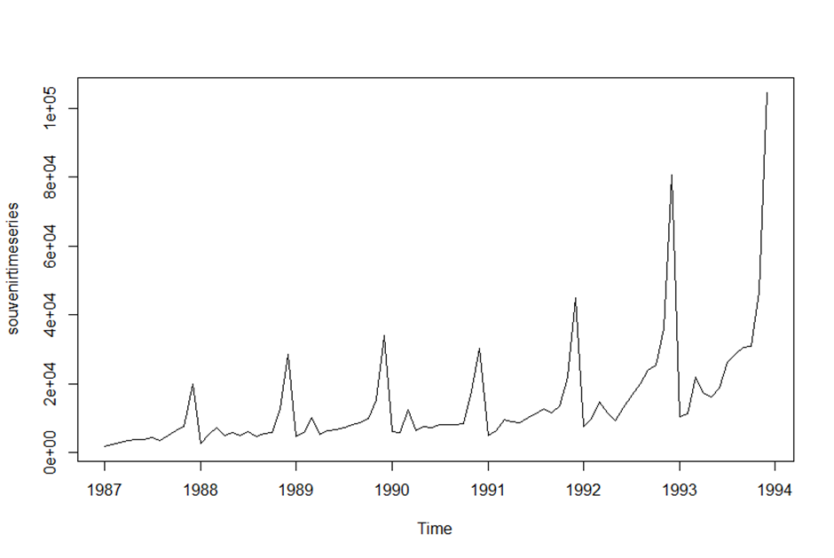
> # 비치 리조트 기념품 매장의 매출액 데이터(1987.01~1993.12)
> souvenir <- scan("https://robjhyndman.com/tsdldata/data/fancy.dat")
Read 84 items
> souvenirtimeseries <- ts(souvenir, frequency = 12, start = c(1987,1))
> souvenirtimeseries
Jan Feb Mar Apr May Jun Jul Aug Sep Oct Nov
1987 1664.81 2397.53 2840.71 3547.29 3752.96 3714.74 4349.61 3566.34 5021.82 6423.48 7600.60
1988 2499.81 5198.24 7225.14 4806.03 5900.88 4951.34 6179.12 4752.15 5496.43 5835.10 12600.08
1989 4717.02 5702.63 9957.58 5304.78 6492.43 6630.80 7349.62 8176.62 8573.17 9690.50 15151.84
1990 5921.10 5814.58 12421.25 6369.77 7609.12 7224.75 8121.22 7979.25 8093.06 8476.70 17914.66
1991 4826.64 6470.23 9638.77 8821.17 8722.37 10209.48 11276.55 12552.22 11637.39 13606.89 21822.11
1992 7615.03 9849.69 14558.40 11587.33 9332.56 13082.09 16732.78 19888.61 23933.38 25391.35 36024.80
1993 10243.24 11266.88 21826.84 17357.33 15997.79 18601.53 26155.15 28586.52 30505.41 30821.33 46634.38
Dec
1987 19756.21
1988 28541.72
1989 34061.01
1990 30114.41
1991 45060.69
1992 80721.71
1993 104660.67
>
> plot.ts(kingstimeseries)

> plot.ts(birthstimeseries)
> plot.ts(souvenirtimeseries)
>
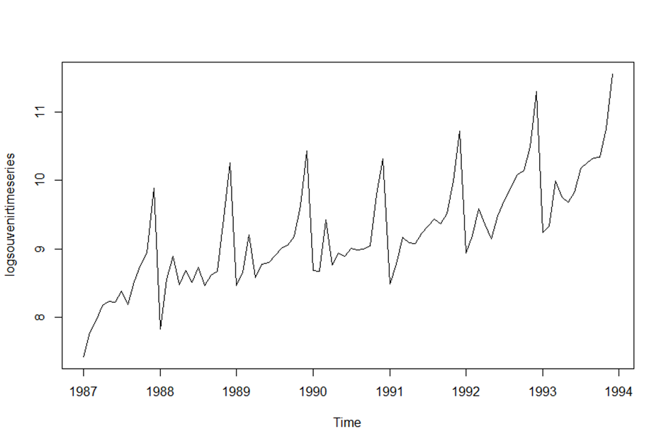
> logsouvenirtimeseries <- log(souvenirtimeseries)
> plot.ts(logsouvenirtimeseries)
>
> kingstimeseriesSMA3 <- SMA(kingstimeseries,n=3)
> plot.ts(kingstimeseriesSMA3)

> # 3년마다 평균을 내서 그래프를 부드럽게 표현
> kingstimeseriesSMA8 <- SMA(kingstimeseries,n=8)
> plot.ts(kingstimeseriesSMA8)
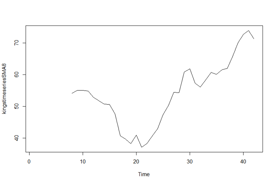
> # 8년마다 평균을 내서 그래프를 더욱 부드로운 곡선으로 표현
>
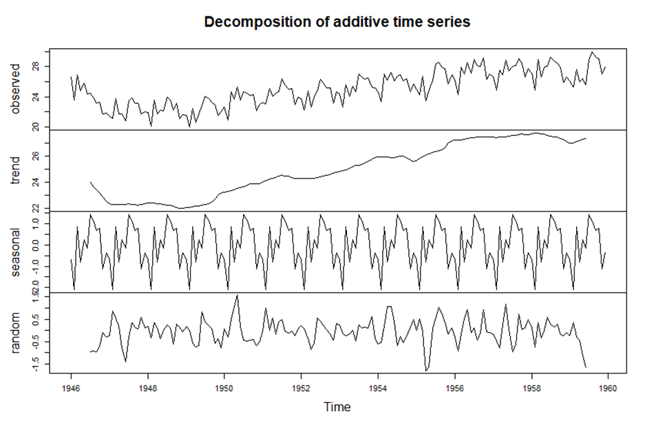
> birthstimeseriescomponents <- decompose(birthstimeseries)
> birthstimeseriescomponents$seasonal
Jan Feb Mar Apr May Jun Jul Aug Sep Oct
1946 -0.6771947 -2.0829607 0.8625232 -0.8016787 0.2516514 -0.1532556 1.4560457 1.1645938 0.6916162 0.7752444
1947 -0.6771947 -2.0829607 0.8625232 -0.8016787 0.2516514 -0.1532556 1.4560457 1.1645938 0.6916162 0.7752444
1948 -0.6771947 -2.0829607 0.8625232 -0.8016787 0.2516514 -0.1532556 1.4560457 1.1645938 0.6916162 0.7752444
1949 -0.6771947 -2.0829607 0.8625232 -0.8016787 0.2516514 -0.1532556 1.4560457 1.1645938 0.6916162 0.7752444
1950 -0.6771947 -2.0829607 0.8625232 -0.8016787 0.2516514 -0.1532556 1.4560457 1.1645938 0.6916162 0.7752444
1951 -0.6771947 -2.0829607 0.8625232 -0.8016787 0.2516514 -0.1532556 1.4560457 1.1645938 0.6916162 0.7752444
1952 -0.6771947 -2.0829607 0.8625232 -0.8016787 0.2516514 -0.1532556 1.4560457 1.1645938 0.6916162 0.7752444
1953 -0.6771947 -2.0829607 0.8625232 -0.8016787 0.2516514 -0.1532556 1.4560457 1.1645938 0.6916162 0.7752444
1954 -0.6771947 -2.0829607 0.8625232 -0.8016787 0.2516514 -0.1532556 1.4560457 1.1645938 0.6916162 0.7752444
1955 -0.6771947 -2.0829607 0.8625232 -0.8016787 0.2516514 -0.1532556 1.4560457 1.1645938 0.6916162 0.7752444
1956 -0.6771947 -2.0829607 0.8625232 -0.8016787 0.2516514 -0.1532556 1.4560457 1.1645938 0.6916162 0.7752444
1957 -0.6771947 -2.0829607 0.8625232 -0.8016787 0.2516514 -0.1532556 1.4560457 1.1645938 0.6916162 0.7752444
1958 -0.6771947 -2.0829607 0.8625232 -0.8016787 0.2516514 -0.1532556 1.4560457 1.1645938 0.6916162 0.7752444
1959 -0.6771947 -2.0829607 0.8625232 -0.8016787 0.2516514 -0.1532556 1.4560457 1.1645938 0.6916162 0.7752444
Nov Dec
1946 -1.1097652 -0.3768197
1947 -1.1097652 -0.3768197
1948 -1.1097652 -0.3768197
1949 -1.1097652 -0.3768197
1950 -1.1097652 -0.3768197
1951 -1.1097652 -0.3768197
1952 -1.1097652 -0.3768197
1953 -1.1097652 -0.3768197
1954 -1.1097652 -0.3768197
1955 -1.1097652 -0.3768197
1956 -1.1097652 -0.3768197
1957 -1.1097652 -0.3768197
1958 -1.1097652 -0.3768197
1959 -1.1097652 -0.3768197
> plot(birthstimeseriescomponents)
>
> birthstimeseriesseasonallyadjusted <- birthstimeseries - birthstimeseriescomponents$seasonal
> plot(birthstimeseriesseasonallyadjusted)
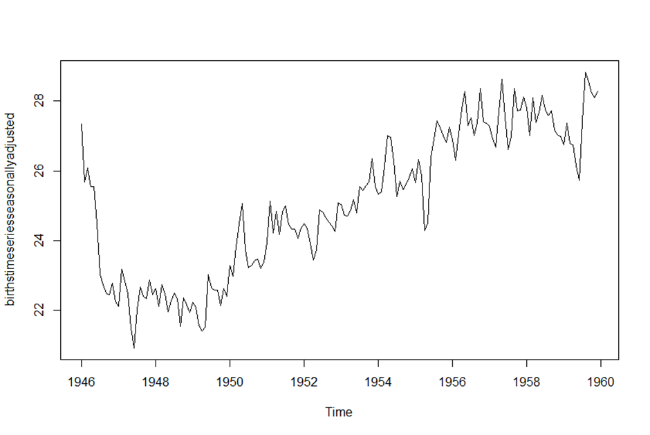
> # 계절성 요소가 제거된 뉴욕 출생자 수 데이터 그래프
>
>
> ## ARIMA 모델
>
> # 매년 여성의 스커트 지름길이 데이터(1866~1911)
> skirts <- scan("https://robjhyndman.com/tsdldata/roberts/skirts.dat",skip = 5)
Read 46 items
> skirtsseries <- ts(skirts,start = c(1866))
> plot.ts(skirtsseries)

> # 시간에 의존적인 비정상시계열
>
> # 차분 후 그래프
> skirtsseriesdiff1 <- diff(skirtsseries, differences = 1)
> plot.ts(skirtsseriesdiff1)

> # 아직 시간이 지남에 따라 평균이 일정치 않음
> skirtsseriesdiff2 <- diff(skirtsseries, differences = 2)
> plot.ts(skirtsseriesdiff2)

> # 차분을 2번 한 결과 평균과 분산이 시간에 의존해 변하지 않는 정상성이 만족된 모습이다.
>
> kings <- scan("https://robjhyndman.com/tsdldata/misc/kings.dat", skip = 3)
Read 42 items
> kingstimeseries <- ts(kings)
> kingstimeseriesdiff1 <- diff(kingstimeseries, differences = 1)
> plot.ts(kingstimeseriesdiff1)
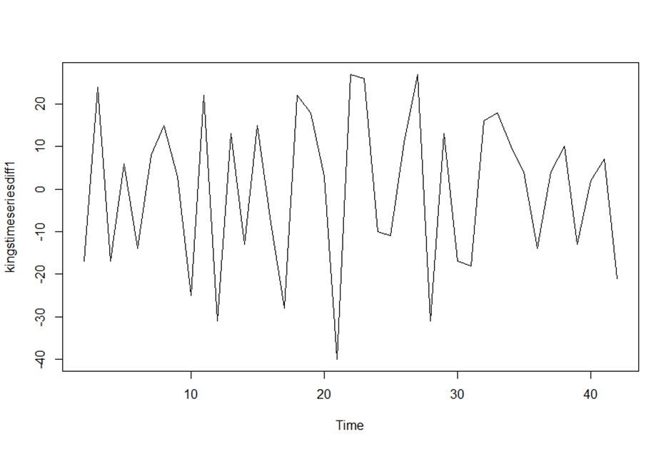
> # 첫번째 차분 결과에서 평균과 분신이 시간에 따라 의존하지 않음을 확인할 수 있다.
> # 즉 ARIMA(p,1,q) 모델이며, 차분을 1번 해야 정상성을 만족한다.
>
>
> ## 적합한 ARIMA 모델 결정
>
> acf(kingstimeseriesdiff1, lag.max = 20)

> acf(kingstimeseriesdiff1, lag.max = 20, plot = FALSE)
Autocorrelations of series ‘kingstimeseriesdiff1’, by lag
0 1 2 3 4 5 6 7 8 9 10 11 12 13 14 15 16
1.000 -0.360 -0.162 -0.050 0.227 -0.042 -0.181 0.095 0.064 -0.116 -0.071 0.206 -0.017 -0.212 0.130 0.114 -0.009
17 18 19 20
-0.192 0.072 0.113 -0.093
> # lag가 1인 지점 빼고는 모두 점선 구간 안에 있고, 나머지는 구간 안에 있음을 확인했다.
>
> pacf(kingstimeseriesdiff1, lag.max = 20)
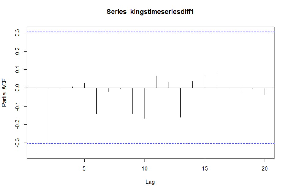
> pacf(kingstimeseriesdiff1, lag.max = 20, plot = FALSE)
Partial autocorrelations of series ‘kingstimeseriesdiff1’, by lag
1 2 3 4 5 6 7 8 9 10 11 12 13 14 15 16 17
-0.360 -0.335 -0.321 0.005 0.025 -0.144 -0.022 -0.007 -0.143 -0.167 0.065 0.034 -0.161 0.036 0.066 0.081 -0.005
18 19 20
-0.027 -0.006 -0.037
> # PACF 값이 lag 1,2,3에서 점선 구간을 초과하고 음의 값을 가지며 절단점이 lag4임을 볼 수 있다.
>
> # 종합해 보면 다음과 같은 ARMA 후보들이 생성된다.
> # - ARMA(3,0) 모형 : PACF 값이 lag 4에서 절단점을 가짐
> # - ARMA(0,1) 모형 : ACF 값이 lag 2에서 절단점을 가짐
> # - ARMA(p,q) 모형 : 그래서 AR 모형과 MA 모형을 혼합함
> # 모델링의 기본은 모수(parameter)들이 적으면 적을수록 단순하고 이해하기 쉽다.
> # 이들 중에서 가장 간단하고 표현하기 쉬운 모형은 ARMA(0,1) 모형이다. 즉 MA(1) 모형으로 최종 결정할 수 있다.
>
> auto.arima(kings)
Series: kings
ARIMA(0,1,1)
Coefficients:
ma1
-0.7218
s.e. 0.1208
sigma^2 estimated as 236.2: log likelihood=-170.06
AIC=344.13 AICc=344.44 BIC=347.56
> # 위의 결과에서 영국 왕의 사망 나이 데이터의 적절한 ARIMA 모형은 ARIMA(0,1,1)임을 알 수 있다.
>
>
> # 화산폭발 먼지량 데이터(1500~1969)
> volcanodust <- scan("https://robjhyndman.com/tsdldata/annual/dvi.dat",skip = 1)
Read 470 items
> volcanodustseries <- ts(volcanodust, start = c(1500))
> plot.ts(volcanodustseries)
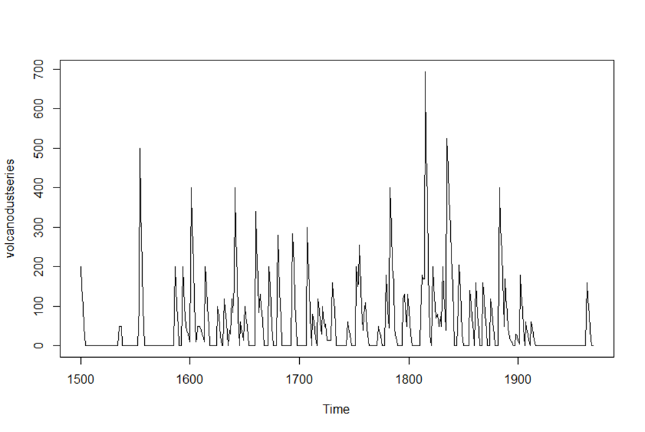
> # 평균과 분산이 시간에 따라 의존하지 않으므로 정상성을 만족한다. 즉 이 데이터는 차분하지 않아도 된다.
>
> acf(volcanodustseries, lag.max = 20)
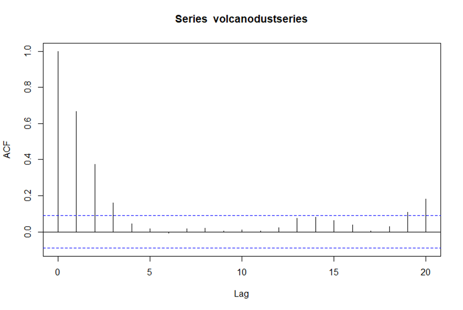
> acf(volcanodustseries, lag.max = 20, plot = FALSE)
Autocorrelations of series ‘volcanodustseries’, by lag
0 1 2 3 4 5 6 7 8 9 10 11 12 13 14 15 16
1.000 0.666 0.374 0.162 0.046 0.017 -0.007 0.016 0.021 0.006 0.010 0.004 0.024 0.075 0.082 0.064 0.039
17 18 19 20
0.005 0.028 0.108 0.182
> # ACF 값이 Lag 1,2,3 지점에서 점선을 초과하고, 나머지는 대부분 점선 안에 있다.
> # Lag19와 20에서 ACF값이 점선을 초과하지만 95% 신뢰구간에서 오차로 인한 부분일 가능성이 크므로 무시할 수 있다.
>
> pacf(volcanodustseries, lag.max = 20)

> pacf(volcanodustseries, lag.max = 20, plot = FALSE)
Partial autocorrelations of series ‘volcanodustseries’, by lag
1 2 3 4 5 6 7 8 9 10 11 12 13 14 15 16 17
0.666 -0.126 -0.064 -0.005 0.040 -0.039 0.058 -0.016 -0.025 0.028 -0.008 0.036 0.082 -0.025 -0.014 0.008 -0.025
18 19 20
0.073 0.131 0.063
> # PACF 그래프에서 lag1과 2에서만 신뢰구간을 초과한 것을 볼 수 있다.
>
> # 종합해 보면 다음과 같은 ARMA 후보들이 생성된다.
> # - ARMA(2,0) 모형 : ACF 값은 급격히 감소하고 PACF의 절단점은 3이기 때문임
> # - ARMA(0,3) 모형 : ACF 값이 3 이후로 절단점을 가지며 PACF 값은 급격히 감소하기 때문임
> # - ARMA(p,q) 모형 : AR 모형과 MA 모형의 혼합
>
> auto.arima(volcanodustseries)
Series: volcanodustseries
ARIMA(1,0,2) with non-zero mean
Coefficients:
ar1 ma1 ma2 mean
0.4723 0.2694 0.1279 57.5178
s.e. 0.0936 0.0969 0.0752 8.4883
sigma^2 estimated as 4897: log likelihood=-2661.84
AIC=5333.68 AICc=5333.81 BIC=5354.45
> # auto.arima 함수를 이용한 결과 ARIMA(1,0,2) 모델이 가장 최적이라고 결정됐다.
> # 하지만 ARIMA(1,0,2) 모델은 모수가 3개나 필요한 경우다.
> # 앞에 제시한 모형과 비교해봤을 때 가장 간단한 모형은 ARMA(2,0) 모형으로 판단된다.
> # 일반적으로 미세한 차이로 약간의 오차가 발생해도 모수를 적게 사용한 모델링 보정(fitting)이 적절하다면,
> # 간단하고 이해하기 쉬운 모델을 선택하는 것이 관례적이다. 여기선 ARMA(2,0)을 채택하겠다.
>
>
> ## ARIMA 모델을 이용한 예측
>
> kingstimeseriesarima <- arima(kingstimeseries, order = c(0,1,1))
> kingstimeseriesarima
Call:
arima(x = kingstimeseries, order = c(0, 1, 1))
Coefficients:
ma1
-0.7218
s.e. 0.1208
sigma^2 estimated as 230.4: log likelihood = -170.06, aic = 344.13
> kings
[1] 60 43 67 50 56 42 50 65 68 43 65 34 47 34 49 41 13 35 53 56 16 43 69 59 48 59 86 55 68 51 33 49 67 77 81 67 71 81 68 70
[41] 77 56
> # 42명의 영국 왕 가운데 마지막 왕의 사망 시 나이는 56세임을 알 수 있다.
>
> kingstimeseriesforecasts <- forecast(kingstimeseriesarima)
> kingstimeseriesforecasts
Point Forecast Lo 80 Hi 80 Lo 95 Hi 95
43 67.75063 48.29647 87.20479 37.99806 97.50319
44 67.75063 47.55748 87.94377 36.86788 98.63338
45 67.75063 46.84460 88.65665 35.77762 99.72363
46 67.75063 46.15524 89.34601 34.72333 100.77792
47 67.75063 45.48722 90.01404 33.70168 101.79958
48 67.75063 44.83866 90.66260 32.70979 102.79146
49 67.75063 44.20796 91.29330 31.74523 103.75603
50 67.75063 43.59372 91.90753 30.80583 104.69543
51 67.75063 42.99472 92.50653 29.88974 105.61152
52 67.75063 42.40988 93.09138 28.99529 106.50596
> # 신뢰구간은 80%~95% 사이다.
> plot(kingstimeseriesforecasts)

>
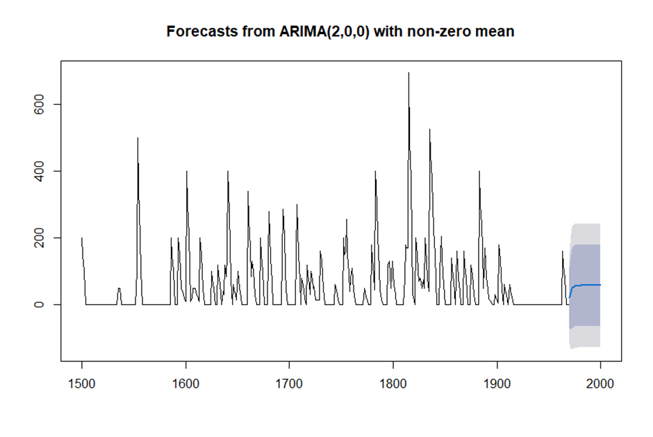
> volcanodustseriesarima <- arima(volcanodustseries, order = c(2,0,0))
> volcanodustseriesarima
Call:
arima(x = volcanodustseries, order = c(2, 0, 0))
Coefficients:
ar1 ar2 intercept
0.7533 -0.1268 57.5274
s.e. 0.0457 0.0458 8.5958
sigma^2 estimated as 4870: log likelihood = -2662.54, aic = 5333.09
> volcanodustseriesforecasts <- forecast(volcanodustseriesarima,h=31)
> volcanodustseriesforecasts
Point Forecast Lo 80 Hi 80 Lo 95 Hi 95
1970 21.48131 -67.94860 110.9112 -115.2899 158.2526
1971 37.66419 -74.30305 149.6314 -133.5749 208.9033
1972 47.13261 -71.57070 165.8359 -134.4084 228.6737
1973 52.21432 -68.35951 172.7881 -132.1874 236.6161
1974 54.84241 -66.22681 175.9116 -130.3170 240.0018
1975 56.17814 -65.01872 177.3750 -129.1765 241.5327
1976 56.85128 -64.37798 178.0805 -128.5529 242.2554
1977 57.18907 -64.04834 178.4265 -128.2276 242.6057
1978 57.35822 -63.88124 178.5977 -128.0615 242.7780
1979 57.44283 -63.79714 178.6828 -127.9777 242.8634
1980 57.48513 -63.75497 178.7252 -127.9356 242.9059
1981 57.50627 -63.73386 178.7464 -127.9145 242.9271
1982 57.51684 -63.72330 178.7570 -127.9040 242.9376
1983 57.52212 -63.71802 178.7623 -127.8987 242.9429
1984 57.52476 -63.71538 178.7649 -127.8960 242.9456
1985 57.52607 -63.71407 178.7662 -127.8947 242.9469
1986 57.52673 -63.71341 178.7669 -127.8941 242.9475
1987 57.52706 -63.71308 178.7672 -127.8937 242.9479
1988 57.52723 -63.71291 178.7674 -127.8936 242.9480
1989 57.52731 -63.71283 178.7674 -127.8935 242.9481
1990 57.52735 -63.71279 178.7675 -127.8934 242.9481
1991 57.52737 -63.71277 178.7675 -127.8934 242.9482
1992 57.52738 -63.71276 178.7675 -127.8934 242.9482
1993 57.52739 -63.71275 178.7675 -127.8934 242.9482
1994 57.52739 -63.71275 178.7675 -127.8934 242.9482
1995 57.52739 -63.71275 178.7675 -127.8934 242.9482
1996 57.52739 -63.71275 178.7675 -127.8934 242.9482
1997 57.52739 -63.71275 178.7675 -127.8934 242.9482
1998 57.52739 -63.71275 178.7675 -127.8934 242.9482
1999 57.52739 -63.71275 178.7675 -127.8934 242.9482
2000 57.52739 -63.71275 178.7675 -127.8934 242.9482
> plot(volcanodustseriesforecasts)
출처 : 데이터 분석 전문가 가이드
'데이터분석 > R' 카테고리의 다른 글
| [현장에서 바로 써먹는...] 정규분포와 중심극한정리 (0) | 2022.04.02 |
|---|---|
| [현장에서 바로 써먹는...] 기초통계량 (0) | 2022.04.02 |
| [실무 프로젝트로 배우는...] 마켓 데이터 분석 (0) | 2022.02.08 |
| [실무 프로젝트로 배우는...] 리뷰 데이터 분석을 통한 감성사전 만들기 (0) | 2022.02.05 |
| [실무 프로젝트로 배우는...] 마케팅의 RFM 분석 (0) | 2022.02.02 |


