[실무 프로젝트로 배우는...] 마켓 데이터 분석
> ## 8. 마켓 데이터 분석
>
> ### 8.2 데이터 전처리
>
> #### 8.2.1 데이터 및 패키지 불러오기
>
> library(dplyr)
> library(data.table)
> library(ggplot2)
> library(reshape)
>
> # 다운로드 URL : https://www.kaggle.com/psparks/instacart-market-basket-analysis
> DIR = "F:/1_Study/1_BigData/12_R/02_Practical-R/MarketData/"
> LISTFILES = list.files(DIR)
>
> for(k in 1:length(LISTFILES)) {
+ assign(gsub(".csv","",LISTFILES[k]),
+ fread(paste0(DIR,LISTFILES[k])))
+ }
>
>
> ### 8.3 상위 판매 상품 분석
>
> #### 8.3.1 판매 상품 분석
>
> # 구매/재구매 상품 분석
>
> Order_Id = order_products__prior %>%
+ group_by(order_id) %>%
+ summarise(Count = n(),
+ Reordered = sum(reordered))
>
> nrow(Order_Id)
[1] 3214874
> summary(Order_Id$Count)
Min. 1st Qu. Median Mean 3rd Qu. Max.
1.00 5.00 8.00 10.09 14.00 145.00
> summary(Order_Id$Reordered)
Min. 1st Qu. Median Mean 3rd Qu. Max.
0.000 2.000 4.000 5.949 8.000 130.000
>
> Order_Id$Reorder_Perc = Order_Id$Reordered / Order_Id$Count * 100
> summary(Order_Id$Reorder_Perc)
Min. 1st Qu. Median Mean 3rd Qu. Max.
0.00 33.33 66.67 59.87 90.91 100.00
>
> ggplot(Order_Id) +
+ geom_histogram(aes(x = Reorder_Perc), binwidth = 5) +
+ xlab("Reorder Proportion") + ylab("Count") +
+ theme_bw()

>
> Order_products_Department = order_products__prior %>%
+ inner_join(products, by = "product_id") %>%
+ inner_join(departments, by = "department_id")
>
> # 상품 카테고리별 판매 분석
>
> Order_ID_Department = Order_products_Department %>%
+ group_by(department) %>%
+ summarise(Count = n(),
+ Reordered = sum(reordered)) %>%
+ mutate(NonReorder = Count - Reordered,
+ Reorder_Perc = Reordered/Count * 100)
>
> knitr::kable(Order_ID_Department %>%
+ arrange(-Count))
|department | Count| Reordered| NonReorder| Reorder_Perc|
|:---------------|-------:|---------:|----------:|------------:|
|produce | 9479291| 6160710| 3318581| 64.99125|
|dairy eggs | 5414016| 3627221| 1786795| 66.99687|
|snacks | 2887550| 1657973| 1229577| 57.41798|
|beverages | 2690129| 1757892| 932237| 65.34601|
|frozen | 2236432| 1211890| 1024542| 54.18855|
|pantry | 1875577| 650301| 1225276| 34.67205|
|bakery | 1176787| 739188| 437599| 62.81409|
|canned goods | 1068058| 488535| 579523| 45.74049|
|deli | 1051249| 638864| 412385| 60.77190|
|dry goods pasta | 866627| 399581| 467046| 46.10761|
|household | 738666| 297075| 441591| 40.21777|
|breakfast | 709569| 398013| 311556| 56.09222|
|meat seafood | 708931| 402442| 306489| 56.76744|
|personal care | 447123| 143584| 303539| 32.11286|
|babies | 423802| 245369| 178433| 57.89708|
|international | 269253| 99416| 169837| 36.92289|
|alcohol | 153696| 87595| 66101| 56.99237|
|pets | 97724| 58760| 38964| 60.12853|
|missing | 69145| 27371| 41774| 39.58493|
|other | 36291| 14806| 21485| 40.79799|
|bulk | 34573| 19950| 14623| 57.70399|
>
> # 카테고리별 판매량
> Order_ID_Department %>%
+ select(department, NonReorder, Reordered) %>%
+ as.data.frame() %>%
+ melt(id.vars = c("department")) %>%
+ ggplot() +
+ geom_bar(aes(x = reorder(department,value), y = value, fill = variable), stat = 'identity') +
+ xlab("Department") + ylab("Sales Count") +
+ labs(fill = "") +
+ coord_flip() +
+ theme_bw() +
+ theme(legend.position = "bottom")
경고메시지(들):
In melt(., id.vars = c("department")) :
The melt generic in data.table has been passed a data.frame and will attempt to redirect to the relevant reshape2 method; please note that reshape2 is deprecated, and this redirection is now deprecated as well. To continue using melt methods from reshape2 while both libraries are attached, e.g. melt.list, you can prepend the namespace like reshape2::melt(.). In the next version, this warning will become an error.

>
> # 카테고리별 재구매 비율
> Order_ID_Department %>%
+ ggplot() +
+ geom_bar(aes(x = reorder(department, Reorder_Perc), y = Reorder_Perc), stat = 'identity') +
+ geom_label(aes(x = reorder(department, Reorder_Perc), y = Reorder_Perc,
+ label = round(Reorder_Perc,2))) +
+ xlab("Department") + ylab("Reorder Percent (%)") +
+ labs(fill = "") +
+ coord_flip() +
+ theme_bw()

>
> # 세부 상품별 판매 분석
>
> Order_ID_Product = Order_products_Department %>%
+ group_by(department, product_name) %>%
+ summarise(Count = n(),
+ Reordered = sum(reordered)) %>%
+ mutate(NonReorder = Count - Reordered,
+ Reorder_Perc = Reordered/Count * 100)
`summarise()` has grouped output by 'department'. You can override using the `.groups` argument.
>
> Order_ID_Product %>%
+ ungroup() %>%
+ top_n(n = 10, wt = Count)
# A tibble: 10 x 6
department product_name Count Reordered NonReorder Reorder_Perc
<chr> <chr> <int> <int> <int> <dbl>
1 dairy eggs Organic Whole Milk 137905 114510 23395 83.0
2 produce Bag of Organic Bananas 379450 315913 63537 83.3
3 produce Banana 472565 398609 73956 84.4
4 produce Large Lemon 152657 106255 46402 69.6
5 produce Limes 140627 95768 44859 68.1
6 produce Organic Avocado 176815 134044 42771 75.8
7 produce Organic Baby Spinach 241921 186884 55037 77.3
8 produce Organic Hass Avocado 213584 170131 43453 79.7
9 produce Organic Strawberries 264683 205845 58838 77.8
10 produce Strawberries 142951 99802 43149 69.8
>
> # 특정 카테고리의 상품별 판매량 그래프 함수 정의
> Product_Graph = function(Order_ID_Product, department_name) {
+
+ Graph = Order_ID_Product %>%
+ dplyr::filter(department == department_name) %>%
+ ungroup() %>%
+ top_n(n = 20, wt = Count) %>%
+ select(department, product_name, NonReorder, Reordered) %>%
+ as.data.frame() %>%
+ melt(id.vars = c("department","product_name")) %>%
+ ggplot() +
+ geom_bar(aes(x = reorder(product_name,value), y = value, fill = variable), stat = 'identity') +
+ xlab("product name") + ylab("Sales Count") +
+ labs(fill = "") +
+ coord_flip() +
+ theme_bw() +
+ theme(legend.position = "bottom") +
+ ggtitle(department_name)
+
+ return(Graph)
+
+ }
>
> Product_Graph(Order_ID_Product = Order_ID_Product,
+ department_name = "snacks")
경고메시지(들):
In melt(., id.vars = c("department", "product_name")) :
The melt generic in data.table has been passed a data.frame and will attempt to redirect to the relevant reshape2 method; please note that reshape2 is deprecated, and this redirection is now deprecated as well. To continue using melt methods from reshape2 while both libraries are attached, e.g. melt.list, you can prepend the namespace like reshape2::melt(.). In the next version, this warning will become an error.

>
>
> ### 8.4 고객 구매 패턴 분석
>
> #### 8.4.1 고객 재방문 시기 분석
>
> orders_prior = orders %>%
+ dplyr::filter(eval_set == "prior")
>
> User_Orders = orders_prior %>%
+ group_by(user_id) %>%
+ summarise(Count = n(),
+ Revisit_Days_Mean = mean(days_since_prior_order, na.rm = TRUE),
+ Revisit_Days_Median = median(days_since_prior_order, na.rm = TRUE),
+ Revisit_Days_Mean = round(Revisit_Days_Mean,2),
+ Revisit_Days_Median = round(Revisit_Days_Median,2))
>
> knitr::kable(User_Orders[1:10,])
| user_id| Count| Revisit_Days_Mean| Revisit_Days_Median|
|-------:|-----:|-----------------:|-------------------:|
| 1| 10| 19.56| 20.0|
| 2| 14| 15.23| 13.0|
| 3| 12| 12.09| 11.0|
| 4| 5| 13.75| 17.0|
| 5| 4| 13.33| 11.0|
| 6| 3| 9.00| 9.0|
| 7| 20| 10.68| 7.0|
| 8| 3| 30.00| 30.0|
| 9| 3| 18.00| 18.0|
| 10| 5| 19.75| 18.5|
>
> User_Orders_Info = orders_prior %>%
+ inner_join(Order_Id, by = "order_id") %>%
+ group_by(user_id) %>%
+ summarise(Count = n(),
+ Revisit_Days_Mean = mean(days_since_prior_order, na.rm = TRUE),
+ Revisit_Days_Median = median(days_since_prior_order, na.rm = TRUE),
+ Revisit_Days_Mean = round(Revisit_Days_Mean,2),
+ Revisit_Days_Median = round(Revisit_Days_Median,2),
+ Reorder_Mean = mean(Reordered))
>
> knitr::kable(User_Orders_Info[1:10,])
| user_id| Count| Revisit_Days_Mean| Revisit_Days_Median| Reorder_Mean|
|-------:|-----:|-----------------:|-------------------:|------------:|
| 1| 10| 19.56| 20.0| 4.1000000|
| 2| 14| 15.23| 13.0| 6.6428571|
| 3| 12| 12.09| 11.0| 4.5833333|
| 4| 5| 13.75| 17.0| 0.2000000|
| 5| 4| 13.33| 11.0| 3.5000000|
| 6| 3| 9.00| 9.0| 0.6666667|
| 7| 20| 10.68| 7.0| 6.9000000|
| 8| 3| 30.00| 30.0| 4.3333333|
| 9| 3| 18.00| 18.0| 6.0000000|
| 10| 5| 19.75| 18.5| 9.8000000|
>
> #### 8.4.2 고객 구매 물품 분석
>
> # 연관분석
>
> # 데이터 무작위 추출
> set.seed(1234)
> Order_id = unique(Order_products_Department$order_id)
> SL = sample(1:length(Order_id), length(Order_id) * 0.1)
> Sample_Order_id = Order_id[SL]
> Sample_Orders = Order_products_Department %>%
+ dplyr::filter(order_id %in% Sample_Order_id)
>
> # 거래행렬 생성
>
> library(arules)
> install.packages("arulesViz")
> library(arulesViz)
>
> DepartmentList = split(Sample_Orders$department, Sample_Orders$order_id)
> DepartmentList_trans = as(DepartmentList, "transactions")
경고메시지(들):
In asMethod(object) : removing duplicated items in transactions
> summary(DepartmentList_trans)
transactions as itemMatrix in sparse format with
321487 rows (elements/itemsets/transactions) and
21 columns (items) and a density of 0.2257279
most frequent items:
produce dairy eggs beverages snacks frozen (Other)
241354 218462 145446 138744 118269 661665
element (itemset/transaction) length distribution:
sizes
1 2 3 4 5 6 7 8 9 10 11 12 13 14 15 16 18
28687 39610 46590 49013 44822 36720 28012 19879 12878 7923 4247 1984 789 262 55 15 1
Min. 1st Qu. Median Mean 3rd Qu. Max.
1.00 3.00 4.00 4.74 6.00 18.00
includes extended item information - examples:
labels
1 alcohol
2 babies
3 bakery
includes extended transaction information - examples:
transactionID
1 11
2 15
3 18
> # most frequent items = 가장 많이 구매한 상품 카테고리
> # includes extended item information = 카테고리에 대한 고유번호
> # transactionID = 구매번호
>
> # 연관분석 진행
>
> rules1 = apriori(DepartmentList_trans,
+ parameter = list(support = 0.2, confidence = 0.1, minlen = 2))
Apriori
Parameter specification:
confidence minval smax arem aval originalSupport maxtime support minlen maxlen target ext
0.1 0.1 1 none FALSE TRUE 5 0.2 2 10 rules TRUE
Algorithmic control:
filter tree heap memopt load sort verbose
0.1 TRUE TRUE FALSE TRUE 2 TRUE
Absolute minimum support count: 64297
set item appearances ...[0 item(s)] done [0.00s].
set transactions ...[21 item(s), 321487 transaction(s)] done [0.08s].
sorting and recoding items ... [9 item(s)] done [0.01s].
creating transaction tree ... done [0.14s].
checking subsets of size 1 2 3 done [0.00s].
writing ... [38 rule(s)] done [0.00s].
creating S4 object ... done [0.03s].
> rules1
set of 38 rules
>
> rule.list1 = as.data.frame(inspect(rules1))
lhs rhs support confidence coverage lift count
[1] {deli} => {produce} 0.2068451 0.8607710 0.2403021 1.1465593 66498
[2] {produce} => {deli} 0.2068451 0.2755206 0.7507426 1.1465593 66498
[3] {bakery} => {dairy eggs} 0.2260465 0.8243735 0.2742039 1.2131418 72671
[4] {dairy eggs} => {bakery} 0.2260465 0.3326482 0.6795360 1.2131418 72671
[5] {bakery} => {produce} 0.2296765 0.8376119 0.2742039 1.1157111 73838
[6] {produce} => {bakery} 0.2296765 0.3059324 0.7507426 1.1157111 73838
[7] {pantry} => {dairy eggs} 0.2697216 0.7751070 0.3479799 1.1406416 86712
[8] {dairy eggs} => {pantry} 0.2697216 0.3969203 0.6795360 1.1406416 86712
[9] {pantry} => {produce} 0.2868701 0.8243870 0.3479799 1.0980954 92225
[10] {produce} => {pantry} 0.2868701 0.3821151 0.7507426 1.0980954 92225
[11] {frozen} => {dairy eggs} 0.2850815 0.7749283 0.3678811 1.1403786 91650
[12] {dairy eggs} => {frozen} 0.2850815 0.4195238 0.6795360 1.1403786 91650
[13] {frozen} => {produce} 0.2990043 0.8127743 0.3678811 1.0826270 96126
[14] {produce} => {frozen} 0.2990043 0.3982780 0.7507426 1.0826270 96126
[15] {beverages} => {snacks} 0.2285878 0.5052597 0.4524164 1.1707491 73488
[16] {snacks} => {beverages} 0.2285878 0.5296661 0.4315696 1.1707491 73488
[17] {beverages} => {dairy eggs} 0.3212416 0.7100573 0.4524164 1.0449149 103275
[18] {dairy eggs} => {beverages} 0.3212416 0.4727367 0.6795360 1.0449149 103275
[19] {beverages} => {produce} 0.3335500 0.7372633 0.4524164 0.9820453 107232
[20] {produce} => {beverages} 0.3335500 0.4442934 0.7507426 0.9820453 107232
[21] {snacks} => {dairy eggs} 0.3224267 0.7471026 0.4315696 1.0994304 103656
[22] {dairy eggs} => {snacks} 0.3224267 0.4744807 0.6795360 1.0994304 103656
[23] {snacks} => {produce} 0.3372827 0.7815257 0.4315696 1.0410035 108432
[24] {produce} => {snacks} 0.3372827 0.4492654 0.7507426 1.0410035 108432
[25] {dairy eggs} => {produce} 0.5524485 0.8129789 0.6795360 1.0828996 177605
[26] {produce} => {dairy eggs} 0.5524485 0.7358693 0.7507426 1.0828996 177605
[27] {dairy eggs,pantry} => {produce} 0.2323422 0.8614148 0.2697216 1.1474169 74695
[28] {pantry,produce} => {dairy eggs} 0.2323422 0.8099214 0.2868701 1.1918741 74695
[29] {dairy eggs,produce} => {pantry} 0.2323422 0.4205681 0.5524485 1.2085990 74695
[30] {dairy eggs,frozen} => {produce} 0.2443489 0.8571195 0.2850815 1.1416955 78555
[31] {frozen,produce} => {dairy eggs} 0.2443489 0.8172087 0.2990043 1.2025980 78555
[32] {dairy eggs,produce} => {frozen} 0.2443489 0.4423017 0.5524485 1.2022953 78555
[33] {beverages,dairy eggs} => {produce} 0.2616809 0.8145921 0.3212416 1.0850484 84127
[34] {beverages,produce} => {dairy eggs} 0.2616809 0.7845326 0.3335500 1.1545121 84127
[35] {dairy eggs,produce} => {beverages} 0.2616809 0.4736747 0.5524485 1.0469883 84127
[36] {dairy eggs,snacks} => {produce} 0.2706983 0.8395655 0.3224267 1.1183133 87026
[37] {produce,snacks} => {dairy eggs} 0.2706983 0.8025860 0.3372827 1.1810793 87026
[38] {dairy eggs,produce} => {snacks} 0.2706983 0.4899975 0.5524485 1.1353847 87026
> rule.list1[order(-rule.list1$support),][1:5,]
lhs rhs support confidence coverage lift count
[25] {dairy eggs} => {produce} 0.5524485 0.8129789 0.6795360 1.0828996 177605
[26] {produce} => {dairy eggs} 0.5524485 0.7358693 0.7507426 1.0828996 177605
[23] {snacks} => {produce} 0.3372827 0.7815257 0.4315696 1.0410035 108432
[24] {produce} => {snacks} 0.3372827 0.4492654 0.7507426 1.0410035 108432
[19] {beverages} => {produce} 0.3335500 0.7372633 0.4524164 0.9820453 107232
>
> # 연관분석 시각화
>
> plot(rules1)

> # 지지도와 신뢰도의 산점도가 출력된다.
>
> # 생성된 규칙을 네트워크 그래프로 표현
> plot(rules1,
+ method = "graph",
+ control = list(type="items"),
+ vertex.label.cex = 0.1,
+ edge.arrow.size = 0.1,
+ edge.arrow.width = 2)
경고: Unknown control parameters: type, vertex.label.cex, edge.arrow.size, edge.arrow.width
Available control parameters (with default values):
layout = stress
circular = FALSE
ggraphdots = NULL
edges = <environment>
nodes = <environment>
nodetext = <environment>
colors = c("#EE0000FF", "#EEEEEEFF")
engine = ggplot2
max = 100
verbose = FALSE

> # 많이 판매되는 상품 카테고리일수록 중앙에 위치한다. (produce, daily eggs 카테고리가 많이 팔리는 것을 확인할 수 있다.)
>
> # 생성된 규칙의 지지도와 향상도를 행렬 형태로 표현
> plot(rules1, method = "grouped matrix")
Registered S3 methods overwritten by 'registry':
method from
print.registry_field proxy
print.registry_entry proxy

> # 7 rules: {produce}은 produce를 구매했을 때 총 7가지{bakery, pantry, deli, dairy eggs, frozen, snacks, beverages} 를 같이 구매했음을 의미한다.
>
> #### 8.4.3 고객의 구매 패턴에 따른 군집 생성
>
> # 고객 패턴 데이터 생성
>
> # reshape 패키지의 cast() 명령어 활용
>
> Orders_Department_Matrix = Order_products_Department %>%
+ slice(1:10000) %>%
+ select(order_id, department) %>%
+ mutate(Count = 1) %>%
+ reshape::cast(order_id~department,
+ fun.aggregate = sum)
Using Count as value column. Use the value argument to cast to override this choice
>
> Orders_Department_Matrix
order_id alcohol babies bakery beverages breakfast bulk canned goods dairy eggs deli dry goods pasta frozen household
1 2 0 0 0 0 0 0 0 1 0 0 0 0
2 3 0 0 1 0 0 0 0 3 0 0 0 0
3 4 0 0 1 3 4 0 0 0 0 0 0 0
4 5 0 0 0 1 0 0 0 3 1 2 0 3
5 6 0 0 0 1 0 0 0 0 0 0 0 2
...
international meat seafood missing other pantry personal care pets produce snacks
1 0 0 0 0 5 0 0 3 0
2 0 1 0 0 0 0 0 3 0
3 0 0 0 0 0 1 0 0 4
4 1 1 0 0 2 1 0 7 4
5 0 0 0 0 0 0 0 0 0
...
[ reached 'max' / getOption("max.print") -- omitted 932 rows ]
> # 이 방법은 대용량의 데이터에 대해서는 연산 속도가 너무 느리기 때문에 추천하는 방법은 아니다.
>
> # tm 패키지의 Corpus(), DocumentMatrix() 명령어 활용
>
> library(tm)
> Order_products_Department$department2 = gsub(" ","",Order_products_Department$department)
>
> Corpus = Corpus(VectorSource(Order_products_Department$department2[1:10000]))
> DTM = DocumentTermMatrix(Corpus)
> DTM_Matrix = as.matrix(DTM)
> DTM_DF = as.data.frame(DTM_Matrix)
> DTM_DF$order_id = Order_products_Department$order_id[1:10000]
> Orders_Department_DF = DTM_DF
>
> # 구매 정보 데이터 생성
>
> set.seed(123)
> SL = sample(1:length(Order_id), length(Order_id) * 0.1)
> Sample_Order_id = Order_id[SL]
> Sample_Orders = Order_products_Department %>%
+ dplyr::filter(order_id %in% Sample_Order_id)
>
> Corpus2 = Corpus(VectorSource(Sample_Orders$department2))
> DTM2 = DocumentTermMatrix(Corpus2)
> DTM_Matrix2 = as.matrix(DTM2)
> DTM_DF2 = as.data.frame(DTM_Matrix2)
> DTM_DF2$order_id = Sample_Orders$order_id
> Orders_Department_DF2 = DTM_DF2
>
> DIR2 = "F:/1_Study/1_BigData/12_R/02_Practical-R/MarketData_output/"
> fwrite(Orders_Department_DF2,
+ paste0(DIR2,"Orders_Department_DF2.csv"))
>
> orders_prior = orders %>%
+ dplyr::filter(eval_set == "prior")
>
> Orders_Department_DF2_Sum = Orders_Department_DF2 %>%
+ group_by(order_id) %>%
+ summarise_all(.funs = sum)
>
> knitr::kable(Orders_Department_DF2_Sum[1:10,])
| order_id| household| produce| bulk| dairyeggs| beverages| babies| international| frozen| cannedgoods| pantry| snacks| meatseafood| deli| drygoodspasta| personalcare| bakery| breakfast| other| alcohol| pets| missing|
|--------:|---------:|-------:|----:|---------:|---------:|------:|-------------:|------:|-----------:|------:|------:|-----------:|----:|-------------:|------------:|------:|---------:|-----:|-------:|----:|-------:|
| 18| 1| 10| 1| 2| 1| 3| 1| 1| 1| 4| 1| 1| 1| 0| 0| 0| 0| 0| 0| 0| 0|
| 28| 0| 6| 0| 8| 0| 0| 0| 0| 0| 1| 0| 1| 0| 0| 0| 0| 0| 0| 0| 0| 0|
| 31| 0| 6| 0| 0| 1| 0| 0| 0| 0| 0| 1| 1| 0| 1| 0| 0| 0| 0| 0| 0| 0|
| 43| 1| 1| 0| 3| 0| 0| 0| 0| 0| 0| 1| 0| 0| 0| 1| 0| 0| 0| 0| 0| 0|
| 51| 1| 4| 0| 1| 1| 0| 0| 0| 0| 1| 0| 0| 0| 0| 0| 1| 0| 0| 0| 0| 0|
| 58| 0| 4| 0| 0| 0| 0| 0| 0| 0| 0| 0| 0| 1| 1| 0| 0| 0| 0| 0| 0| 0|
| 61| 0| 4| 0| 6| 0| 0| 0| 0| 0| 0| 1| 0| 0| 0| 0| 0| 1| 0| 0| 0| 0|
| 79| 2| 1| 0| 1| 3| 0| 0| 0| 0| 0| 0| 0| 0| 0| 0| 0| 0| 1| 0| 0| 0|
| 90| 0| 1| 0| 0| 0| 0| 0| 0| 3| 1| 0| 0| 0| 0| 0| 0| 0| 0| 0| 0| 0|
| 103| 0| 0| 0| 0| 4| 0| 0| 0| 0| 0| 0| 0| 0| 0| 0| 0| 0| 0| 0| 0| 0|
>
> Orders_Department_DF2_User = Orders_Department_DF2_Sum %>%
+ inner_join(orders_prior, by = 'order_id')
>
> User_Orders_Product = Orders_Department_DF2_User %>%
+ select(-eval_set,-order_number,-order_dow,-order_id,
+ -order_hour_of_day,-days_since_prior_order) %>%
+ group_by(user_id) %>%
+ summarise_all(.funs = mean)
>
> User_Orders_Product
# A tibble: 130,875 x 22
user_id household produce bulk dairyeggs beverages babies international frozen cannedgoods pantry snacks meatseafood
<int> <dbl> <dbl> <dbl> <dbl> <dbl> <dbl> <dbl> <dbl> <dbl> <dbl> <dbl> <dbl>
1 1 0.25 0 0 1.25 1.25 0 0 0 0 0.25 2 0
2 2 0 2 0 6 2 0 0 0 0 2 4 0
3 3 1 2 0 3 1 0 0 0 0 0 2 0
4 7 0 2 0 0.667 1.67 0 0 0 0 0 0.667 0.333
5 9 1 2 0 7 1 5 0 1 1 3 7 1
6 11 0 2 0 2 3 0 0 0 0 4 0 0
7 12 0 5 0 1 1 0 0 1 0 1 0 0
8 13 0 2 0 2.2 0 0 0 0 0.2 0.2 0.2 0
9 14 0 1 0 0 0 0 0 2 0.5 2 0 0
10 15 0 0 0 0 1 0 0 0 0 0 2.33 0
# ... with 130,865 more rows, and 9 more variables: deli <dbl>, drygoodspasta <dbl>, personalcare <dbl>, bakery <dbl>,
# breakfast <dbl>, other <dbl>, alcohol <dbl>, pets <dbl>, missing <dbl>
>
> # 군집 분석
>
> Sample_Orders_Info = orders_prior %>%
+ dplyr::filter(order_id %in% Order_id) %>%
+ inner_join(Order_Id, by = "order_id") %>%
+ group_by(user_id) %>%
+ summarise(Count = n(),
+ Revisit_Days_Mean = mean(days_since_prior_order, na.rm = TRUE),
+ Revisit_Days_Mean = round(Revisit_Days_Mean,2),
+ Reorder_Mean = mean(Reordered))
>
> User_Orders_Info2 = Sample_Orders_Info %>%
+ inner_join(User_Orders_Product, by = 'user_id') %>%
+ as.data.frame()
>
> knitr::kable(User_Orders_Info2[1:10,])
| user_id| Count| Revisit_Days_Mean| Reorder_Mean| household| produce| bulk| dairyeggs| beverages| babies| international| frozen| cannedgoods| pantry| snacks| meatseafood| deli| drygoodspasta| personalcare| bakery| breakfast| other| alcohol| pets| missing|
|-------:|-----:|-----------------:|------------:|---------:|-------:|----:|---------:|---------:|------:|-------------:|------:|-----------:|------:|---------:|-----------:|---------:|-------------:|------------:|------:|---------:|-----:|-------:|----:|-------:|
| 1| 10| 19.56| 4.100000| 0.25| 0| 0| 1.2500000| 1.250000| 0| 0| 0| 0.0| 0.25| 2.0000000| 0.0000000| 0.0000000| 0| 0| 0.0| 0.0| 0| 0| 0| 0.0|
| 2| 14| 15.23| 6.642857| 0.00| 2| 0| 6.0000000| 2.000000| 0| 0| 0| 0.0| 2.00| 4.0000000| 0.0000000| 2.0000000| 0| 0| 1.0| 0.0| 0| 0| 0| 0.0|
| 3| 12| 12.09| 4.583333| 1.00| 2| 0| 3.0000000| 1.000000| 0| 0| 0| 0.0| 0.00| 2.0000000| 0.0000000| 0.0000000| 0| 0| 0.0| 0.0| 0| 0| 0| 0.0|
| 7| 20| 10.68| 6.900000| 0.00| 2| 0| 0.6666667| 1.666667| 0| 0| 0| 0.0| 0.00| 0.6666667| 0.3333333| 0.3333333| 0| 0| 0.0| 0.0| 0| 0| 0| 0.0|
| 9| 3| 18.00| 6.000000| 1.00| 2| 0| 7.0000000| 1.000000| 5| 0| 1| 1.0| 3.00| 7.0000000| 1.0000000| 0.0000000| 0| 0| 0.0| 1.0| 0| 0| 0| 0.0|
| 11| 7| 20.50| 4.714286| 0.00| 2| 0| 2.0000000| 3.000000| 0| 0| 0| 0.0| 4.00| 0.0000000| 0.0000000| 0.0000000| 0| 0| 0.0| 0.0| 0| 0| 0| 0.0|
| 12| 5| 25.00| 2.600000| 0.00| 5| 0| 1.0000000| 1.000000| 0| 0| 1| 0.0| 1.00| 0.0000000| 0.0000000| 0.0000000| 1| 1| 0.0| 0.0| 0| 0| 6| 0.0|
| 13| 12| 7.64| 4.333333| 0.00| 2| 0| 2.2000000| 0.000000| 0| 0| 0| 0.2| 0.20| 0.2000000| 0.0000000| 0.0000000| 0| 0| 0.6| 0.2| 0| 0| 0| 0.6|
| 14| 13| 22.08| 5.230769| 0.00| 1| 0| 0.0000000| 0.000000| 0| 0| 2| 0.5| 2.00| 0.0000000| 0.0000000| 0.5000000| 0| 0| 1.5| 0.0| 0| 1| 0| 0.0|
| 15| 22| 10.81| 2.681818| 0.00| 0| 0| 0.0000000| 1.000000| 0| 0| 0| 0.0| 0.00| 2.3333333| 0.0000000| 0.0000000| 0| 0| 0.0| 0.0| 0| 0| 0| 0.0|
>
> # 지금까지 정리한 데이터를 기반으로 유사한 구매패턴을 보이는 고객들을 분류하기 위해 군집분석 진행
>
> # 정규화 후 군집분석
>
> Normalization = function(x){
+ y = (x-min(x))/(max(x)-min(x))
+ return(y)
+ }
>
> rownames(User_Orders_Info2) = User_Orders_Info2$user_id
>
> User_Orders_Info2_2 = User_Orders_Info2 %>%
+ select(-user_id)
>
> User_Orders_Normalization = apply(User_Orders_Info2_2,
+ MARGIN = 2,
+ FUN = Normalization)
>
> User_Orders_Normalization = as.data.frame(User_Orders_Normalization)
>
> library(factoextra)
> library(FactoMineR)
>
> set.seed(123)
> SL = sample(1:nrow(User_Orders_Normalization),
+ nrow(User_Orders_Normalization) * 0.05,
+ replace = FALSE)
>
> k_cluster1 = kmeans(User_Orders_Normalization[SL,], 2, nstart = 25)
>
> fviz_cluster(k_cluster1,
+ data = User_Orders_Normalization[SL,],
+ ellipse.type = "convex",
+ palette = "jco",
+ ggtheme = theme_minimal())

>
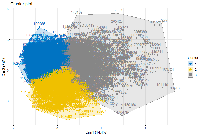
> k_cluster2 = kmeans(User_Orders_Normalization[SL,], 3, nstart = 25)
>
> fviz_cluster(k_cluster2,
+ data = User_Orders_Normalization[SL,],
+ ellipse.type = "convex",
+ palette = "jco",
+ ggtheme = theme_minimal())

>
> # K=2, 3일 때 모두 겹치는 영역이 큰 것을 확인할 수 있다.
>
> # 표준화 후 군집분석
>
> User_Orders_Scale = scale(User_Orders_Info2_2)
> User_Orders_Scale = as.data.frame(User_Orders_Scale)
>
> k_cluster3 = kmeans(User_Orders_Scale[SL,], 2, nstart = 25)
>
> fviz_cluster(k_cluster3,
+ data = User_Orders_Scale[SL,],
+ ellipse.type = "convex",
+ palette = "jco",
+ ggtheme = theme_minimal())

>
> k_cluster4 = kmeans(User_Orders_Scale[SL,], 3, nstart = 25)
>
> fviz_cluster(k_cluster4,
+ data = User_Orders_Scale[SL,],
+ ellipse.type = "convex",
+ palette = "jco",
+ ggtheme = theme_minimal())
>
> # 정규화 후 보다는 겹치는 영역이 눈에 띄게 적다.
>
> # 군집 시각화
>
> Sample_User = User_Orders_Scale[SL,]
> Sample_User = as.data.frame(Sample_User)
> Sample_User$Cluster = k_cluster4$cluster
>
> Sample_User %>%
+ group_by(Cluster) %>%
+ summarise_all(.funs = mean) %>%
+ as.data.frame() %>%
+ melt(id.vars = c("Cluster")) %>%
+ ggplot() +
+ geom_point(aes(x = variable, y = value, col = as.factor(Cluster))) +
+ geom_path(aes(x = variable, y = value, col = as.factor(Cluster),
+ group = as.factor(Cluster))) +
+ labs(col = "Cluster") +
+ xlab("") + ylab("") +
+ coord_polar() +
+ theme_bw() +
+ theme(legend.position = "bottom")
경고메시지(들):
In melt(., id.vars = c("Cluster")) :
The melt generic in data.table has been passed a data.frame and will attempt to redirect to the relevant reshape2 method; please note that reshape2 is deprecated, and this redirection is now deprecated as well. To continue using melt methods from reshape2 while both libraries are attached, e.g. melt.list, you can prepend the namespace like reshape2::melt(.). In the next version, this warning will become an error.

> # 각 군집의 평균값을 레이더 형태로 표현한 그래프이다.
> # 군집 2(초록색)는 Count 변수의 평균이 다른 군집보다 높다.
> # 군집 1(빨간색)의 경우 모든 변수에 대해 대체로 작은 수치로 나타났다.
> # 군집 3(파란색)은 여러 상품 카테고리 구매 빈도가 높다.
>
>
> ### 8.5 추천 시스템
>
> #### 8.5.2 추천 시스템 구현 - 군집분석 기반
>
> install.packages("recommenderlab")
> library(recommenderlab)
>
> rownames(User_Orders_Info2) = User_Orders_Info2$user_id
> User_Orders_Info2_2 = User_Orders_Info2 %>%
+ select(-user_id)
>
> User_Orders_Scale = scale(User_Orders_Info2_2)
> User_Orders_Scale = as.data.frame(User_Orders_Scale)
>
> k_cluster_Total = kmeans(User_Orders_Scale, 3, nstart = 25)
> User_Orders_Info2_2$Cluster = k_cluster_Total$cluster
>
> # 추천 시스템을 위한 데이터 생성
>
> # 추천 시스템을 위한 데이터 생성 - realRatingMatrix
> # 카테고리별 고객의 평균 구매 수량을 평점으로 활용
>
> Cluster3 = User_Orders_Info2_2 %>%
+ dplyr::filter(Cluster == 3) %>%
+ select(-Count,-Revisit_Days_Mean,-Reorder_Mean, -Cluster)
> Cluster3$user_id = paste0("user",rownames(Cluster3))
>
> Cluster3 = Cluster3 %>%
+ melt(id.vars = c("user_id")) %>%
+ arrange(user_id)
경고메시지(들):
In melt(., id.vars = c("user_id")) :
The melt generic in data.table has been passed a data.frame and will attempt to redirect to the relevant reshape2 method; please note that reshape2 is deprecated, and this redirection is now deprecated as well. To continue using melt methods from reshape2 while both libraries are attached, e.g. melt.list, you can prepend the namespace like reshape2::melt(.). In the next version, this warning will become an error.
>
> C3_Matrix = as(Cluster3, "realRatingMatrix")
> head(as(C3_Matrix, "data.frame"))
user item rating
1 user1 household 0
26144 user1 produce 2
52287 user1 bulk 0
78430 user1 dairyeggs 6
104573 user1 beverages 2
130716 user1 babies 0
> C3_DF = as.data.frame(as(C3_Matrix, "data.frame"))
>
> C3_DF$user = as.character(C3_DF$user)
> C3_DF$item = as.character(C3_DF$item)
>
> C3_DF %>%
+ dplyr::filter(user %in% c("user1","user2","user3","user4","user5")) %>%
+ ggplot() +
+ geom_tile(aes(x = user, y = item, fill = rating)) +
+ geom_vline(xintercept = seq(0.5,by = 1, length.out = 9),
+ linetype = 'dashed') +
+ geom_hline(yintercept = seq(0.5,by = 1, length.out = 26),
+ linetype = 'dashed') +
+ scale_fill_gradientn(colours = c("white","black"),
+ values = c(0,0.5,1)) +
+ theme_minimal() +
+ labs(fill = "Rating") +
+ theme(legend.position = "bottom",
+ legend.key.width=unit(3,"cm"),
+ text = element_text(size = 15, face = "bold"),
+ legend.box.background =element_rect())

> # 히트맵으로 고객들의 구매 기록을 시각화
> # 5명의 고객 모두 dairyeggs를 자주 구매한 것을 확인할 수 있다.
>
> C3_Ratings = getRatings(C3_Matrix)
> summary(C3_Ratings)
Min. 1st Qu. Median Mean 3rd Qu. Max.
0.0000 0.0000 0.0000 0.9674 1.0000 44.0000
>
> # 사용자 기반 추천 시스템
>
> SL = 1:round(nrow(C3_Matrix)*0.99)
> C3_Train = C3_Matrix[SL]
> C3_Test = C3_Matrix[-SL]
>
> C3_UBCF = Recommender(C3_Train, method = "UBCF")
>
> C3_U_Predict = predict(C3_UBCF, C3_Test, type="ratingMatrix")
> M3_U = as(C3_U_Predict,"matrix")
> sort(colMeans(M3_U),decreasing = TRUE)
produce dairyeggs snacks frozen beverages pantry cannedgoods bakery
5.849511136 3.653764867 2.165279659 1.657472774 1.275934247 1.213372056 0.840879867 0.721148980
drygoodspasta deli breakfast meatseafood household babies personalcare international
0.706848884 0.662119690 0.468265055 0.399293029 0.240509589 0.210590482 0.143619328 0.129676474
missing pets bulk other alcohol
-0.005934469 -0.020007760 -0.027432865 -0.028609904 -0.030971191
> # 카테고리 추천은 produce, dairyeggs, snacks 순서로 많이 된 것을 확인할 수 있다.
>
> # 개개인에 대한 추천 카테고리
> sort(unlist(as(C3_U_Predict,"list")[1]),decreasing = TRUE)
user9764.frozen user9764.dairyeggs user9764.snacks user9764.produce user9764.drygoodspasta
4.267444070 3.834786840 2.918881010 1.377616208 1.208052726
user9764.pantry user9764.bakery user9764.meatseafood user9764.deli user9764.breakfast
1.124289482 0.665140600 0.437739323 0.326362613 0.314000302
user9764.beverages user9764.cannedgoods user9764.household user9764.international user9764.personalcare
0.297241038 0.086418526 0.036528459 -0.009330444 -0.015894607
user9764.missing user9764.babies user9764.bulk user9764.other user9764.alcohol
-0.029588681 -0.036197060 -0.075872601 -0.075872601 -0.075872601
user9764.pets
-0.075872601
> sort(unlist(as(C3_U_Predict,"list")[2]),decreasing = TRUE)
user9765.snacks user9765.produce user9765.frozen user9765.dairyeggs user9765.pantry
6.1775364 5.8083456 4.1918586 2.7318436 1.6520688
user9765.drygoodspasta user9765.deli user9765.beverages user9765.bakery user9765.meatseafood
1.4238955 1.2085222 1.1048437 1.0807753 1.0002579
user9765.cannedgoods user9765.breakfast user9765.personalcare user9765.international user9765.household
0.7699697 0.7626861 0.6752035 0.5489099 0.5304160
user9765.pets user9765.babies user9765.bulk user9765.other user9765.alcohol
0.4020718 0.4020411 0.3821886 0.3821886 0.3821886
user9765.missing
0.3821886
>
> # 아이템 기반 추천 시스템
>
> C3_IBCF = Recommender(C3_Train, method = "IBCF")
> C3_I_Predict = predict(C3_IBCF, C3_Test, type="ratingMatrix")
> M3_I = as(C3_I_Predict,"matrix")
> sort(colMeans(M3_I),decreasing = TRUE)
cannedgoods drygoodspasta bakery household breakfast deli pets alcohol
1.6912742 1.2811703 1.1946219 1.0324000 1.0263149 1.0187827 1.0123656 1.0078731
other bulk missing personalcare babies international meatseafood dairyeggs
1.0048902 1.0023125 1.0017125 0.9854815 0.9854258 0.9765354 0.9344719 0.6007949
produce snacks beverages pantry frozen
0.3940936 0.3828307 0.3347450 0.1488792 0.1366518
> # 아이템 기반 추천에서는 cannedgoods와 drygoodspasta가 가장 많이 추천된 것을 확인할 수 있다.
>
> # 개개인에 대한 추천 결과
> sort(unlist(as(C3_I_Predict,"list")[1]),decreasing = TRUE)
user9764.cannedgoods user9764.drygoodspasta user9764.international user9764.pets user9764.alcohol
1.530601e+00 8.366094e-01 5.497031e-01 5.478477e-01 5.469612e-01
user9764.bulk user9764.other user9764.missing user9764.deli user9764.household
5.469222e-01 5.467807e-01 5.462298e-01 4.871058e-01 4.839347e-01
user9764.personalcare user9764.babies user9764.meatseafood user9764.bakery user9764.breakfast
4.752139e-01 4.697888e-01 4.658389e-01 4.639385e-01 4.594893e-01
user9764.beverages user9764.snacks user9764.produce user9764.dairyeggs user9764.frozen
4.173209e-01 3.838209e-01 3.168960e-01 1.729550e-01 8.655586e-02
user9764.pantry
1.110223e-16
출처 : 실무 프로젝트로 배우는 데이터 분석 with R