> ## 6 교통 흐름 분석 1 : 통근 시간대
>
>
> # Step 1 : 통근 시간대 교통 흐름 분석
>
> ## 통근 시간대 데이터 필터링
> # 데이터 불러오기
> setwd(dirname(rstudioapi::getSourceEditorContext()$path))
> load("./01_save/04_002_trip_chain.rdata")
> load("./01_save/04_001_sta_pnt.rdata")
> load("./01_save/01_002_fishnet.rdata")
> load("./01_save/01_001_admin.rdata")
> # 통근 통행 필터링 (오전 7,8,9시 + 오후 17,18,19시)
> library(dplyr)
> trip_cmt <- trip_chain[grep("6|7|8|9|17|18|19", trip_chain$start_hour),]
> rownames(trip_cmt) <- 1:nrow(trip_cmt)
> save(trip_cmt, file = "./01_save/06_001_trip_cmt.rdata")
> # trip_cmt에서 필요한 정보만 추출하기
> keeps <- c("id.x", "id.y", "승차역ID1", "최종하차역ID", "총이용객수", "환승횟수")
> grid_chain <- trip_cmt[keeps]
> head(grid_chain)
id.x id.y 승차역ID1 최종하차역ID 총이용객수 환승횟수
1 2630 3185 4100049 4100017 1 1
2 2630 3185 4100049 4100017 1 1
3 2541 3185 4170974 4100017 1 1
4 2630 3185 4100049 4100017 1 1
5 2630 3185 4100049 4100017 1 1
6 2636 3185 4116181 4100017 1 1
> save(grid_chain, file = "./01_save/06_002_grid_chain.rdata")
> rm("trip_chain"); rm("keeps")
>
> ## 집계구 간 이동만 남기기(집계구 내 이동 지우기)
> install.packages("stplanr")
> library(stplanr)
> od_intra <- filter(grid_chain, id.x != id.y)
> # 그리드 간(intra) 이동별 총이용객수, 환승횟수 집계하기
> od_intra2 <- od_intra %>%
+ group_by(id.x, id.y) %>%
+ summarise_each(funs(sum)) %>%
+ dplyr::select(id.x, id.y, 총이용객수, 환승횟수)
Warning messages:
1: `summarise_each_()` was deprecated in dplyr 0.7.0.
Please use `across()` instead.
This warning is displayed once every 8 hours.
Call `lifecycle::last_lifecycle_warnings()` to see where this warning was generated.
2: `funs()` was deprecated in dplyr 0.8.0.
Please use a list of either functions or lambdas:
# Simple named list:
list(mean = mean, median = median)
# Auto named with `tibble::lst()`:
tibble::lst(mean, median)
# Using lambdas
list(~ mean(., trim = .2), ~ median(., na.rm = TRUE))
This warning is displayed once every 8 hours.
Call `lifecycle::last_lifecycle_warnings()` to see where this warning was generated.
> # 평균 환승횟수 계산
> od_intra2$평균환승 <- round((od_intra2$환승횟수 / od_intra2$총이용객수), 1)
> # 컬럼 이름 정리하기
> colnames(od_intra2) <- c("id.x", "id.y", "총이용객수", "환승횟수", "평균환승")
> head(od_intra2)
# A tibble: 6 x 5
# Groups: id.x [2]
id.x id.y 총이용객수 환승횟수 평균환승
<int> <int> <dbl> <dbl> <dbl>
1 1348 2357 8 24 3
2 1348 2637 2 4 2
3 1349 2541 16 24 1.5
4 1349 2544 32 32 1
5 1349 2545 32 32 1
6 1349 2633 8 8 1
>
> ## 시각화 위하여 공간 데이터 형식(OD2LINE)으로 변경
> # 공간 데이터 형식(OD2LINE) 만들기
> od_line <- od2line(od_intra2, as(fishnet, "sf"))
Creating centroids representing desire line start and end points.
> # 저장
> save(od_line, file = "./01_save/06_003_od_line.rdata")
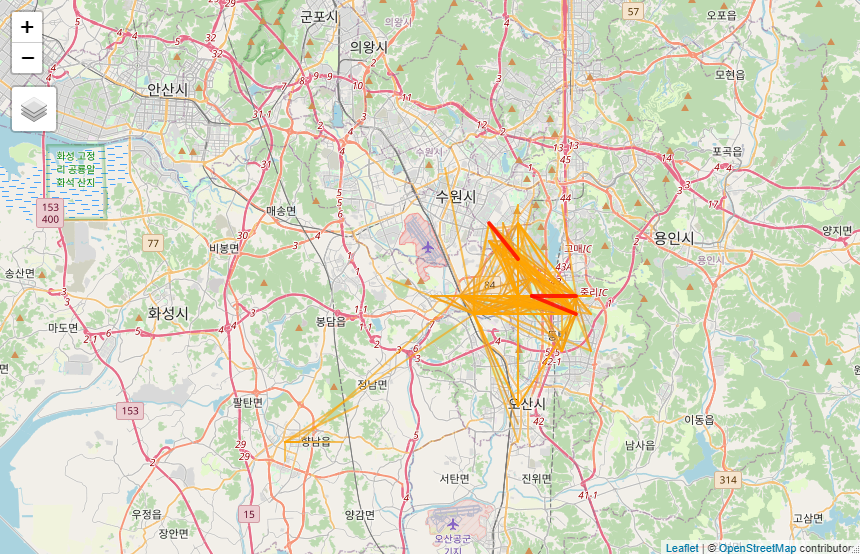
> # 총이용객수 시각화
> library(tmap)
> qtm("Hwaseong")
Switching to view mode. Run tmap_mode("plot") or simply ttm() to switch back to plot mode.
> qtm("Hwaseong") +
+ tm_basemap("OpenStreetMap") +
+ qtm(subset(od_line, od_line$총이용객수 > 30), lines.col = "grey", lines.lwd = .3) +
+ qtm(subset(od_line, od_line$총이용객수 > 100), lines.col = "blue", lines.alpha = .4, lines.lwd = 1) +
+ qtm(subset(od_line, od_line$총이용객수 > 40), lines.col = "orange", lines.alpha = .6, lines.lwd = 2) +
+ qtm(subset(od_line, od_line$총이용객수 > 1000), lines.col = "red", lines.alpha = .8, lines.lwd = 4)
Warning message:
qtm called without shape objects cannot be stacked

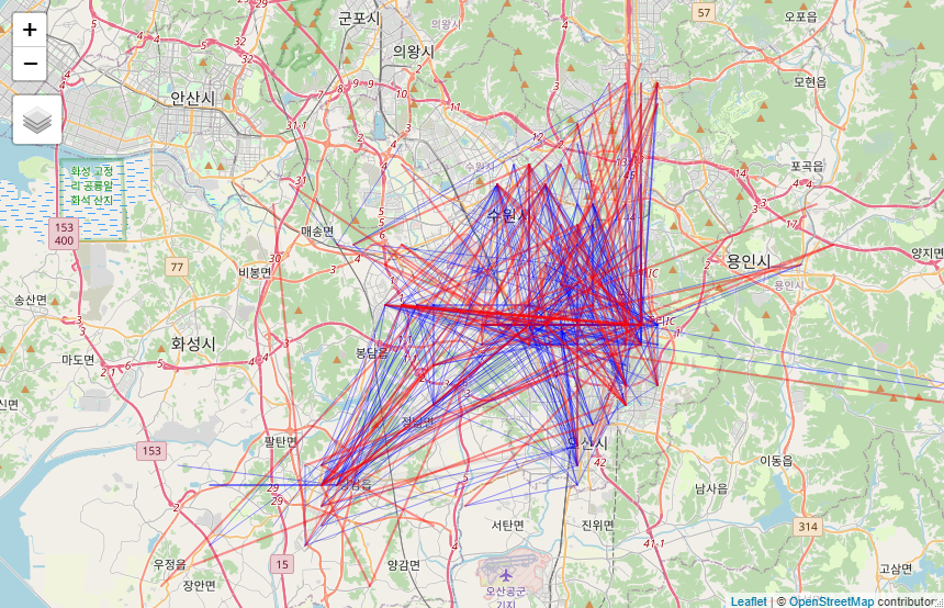
> # 평균환승 시각화
> qtm("Hwaseong")
> qtm("Hwaseong") +
+ tm_basemap("OpenStreetMap") +
+ qtm(subset(od_line, od_line$평균환승 >= 2 & od_line$평균환승 < 3), lines.col = "grey", lines.lwd = .3) +
+ qtm(subset(od_line, od_line$평균환승 >= 3 & od_line$평균환승 < 4), lines.col = "blue", lines.alpha = .4, lines.lwd = 1) +
+ qtm(subset(od_line, od_line$평균환승 >= 4 & od_line$평균환승 < 5), lines.col = "red", lines.alpha = .4, lines.lwd = 2)
Warning message:
qtm called without shape objects cannot be stacked
>
>
> # Step 2 : 통근 시간대 커뮤니티 탐지
>
> # 커뮤니티 탐지(Coummunity Detection)는 네트워크 분석 기법을 이용하여 동질성이 높은 공간 영역을 탐지하는 분석 기법이다.
> # 이를 위해서는 이동 데이터를 네트워크 데이터로 변환하는 과정이 필요하다.
>
> ## 네트워크 속성 변환 (Spatial_data_frame => Spatial_Network)
> library(stplanr)
> # 네트워크 데이터로 변환
> od_line_sln <- SpatialLinesNetwork(od_line)
> # g, nb 등 확인
> head(od_line_sln@nb, 2)
[[1]]
[1] 1 2 575
[[2]]
[1] 1 17 24 29 33 35 38 48 64 91 124 136 165 167 171 187 224 232 238 243 266 279 308
[24] 314 336 362 407 429 430 431 432 433 434 435 436 437 438 439 440 441 442 443 444 445 446 447
[47] 448 449 450 451 452 453 454 455 456 457 458 459 460 461 462 463 464 465 466 467 468 469 470
[70] 520 580 604 632 667 702 736 792 867 920 965 1007 1059 1158 1238 1291 1351 1403 1448 1621 1686 1754
> head(od_line_sln@g, 2)
2 x 159 sparse Matrix of class "dgCMatrix"
[1,] . 12516.12 15592.444 . . . . . . . . . . . .
[2,] 12516.12 . 9731.382 . 4447.804 6928.928 8364.475 3335.853 . 12324.03 . 8923.822 3776.86 8528.92 11967.22
[1,] . . . . . . . . . . . . . . . .
[2,] 2842.681 1770.737 2842.827 . 10361.78 20325.65 2842.9 7107.799 10615 . 10941.88 6902.783 8939.513 . 7783.657 .
[1,] 14360.67 . . . . . . . . . . . . . . . . . . . .
[2,] 2879.63 . 7982.715 7180.595 . 2842.9 . 8528.92 . 18016.16 . 6730.15 . . . . 7105.971 . 5759.585 4182.237 6928.928
[1,] . . . . . . . . . . . . . . . .
[2,] . 6161.258 . . 4954.582 4787.411 . . 7554.051 4535.022 8895.608 5543.704 9070.044 5180.166 5684.923 6902.603
[1,] . . . . . . . . . . . . . . . .
[2,] 3335.853 3451.301 4263.802 . . . 10681.75 12591.46 10853.3 11721.17 4447.804 10683.15 2842.608 . 4954.582 2393.619
[1,] . . . . . . . . . . . . . . . . . . . . . . . . .
[2,] 3463.924 . . 4181.641 . 2656.106 . 8895.608 2223.902 . . . . . . 7833.896 10007.56 4787.411 22239.02 . . . . . .
[1,] . . . . . . . . . . . . . . . . . . . . . . . . . . . . . . . . . . . . . . . . . . . . . . . . . .
[2,] 8939.606 . 12445.75 . . . . . . . . . . . . . . . . . . . . . . . . . . . . . . . . . . . . . . . . . . . . . . .
> # 네트워크 가중치 부여하기
> library(igraph)
> E(od_line_sln@g)$weight <- od_line$총이용객수
> # 엣지 속성 보기
> edge_attr(od_line_sln@g)$weight
[1] 8 2 16 32 32 8 4 6 2 2 16 6 8 4 6 1 4 4 1 8 8 2 2
[24] 4 6 6 2 1 8 4 1 1 40 3 4 1 15 24 1 2 14 16 32 6 4 4
[47] 9 12 1 1 2 2 6 8 1 8 4 2 1 1 3 2 2 24 1 12 4 1 1
...
[990] 3 6 16 3 16 6 24 9 4 6 107
[ reached getOption("max.print") -- omitted 803 entries ]
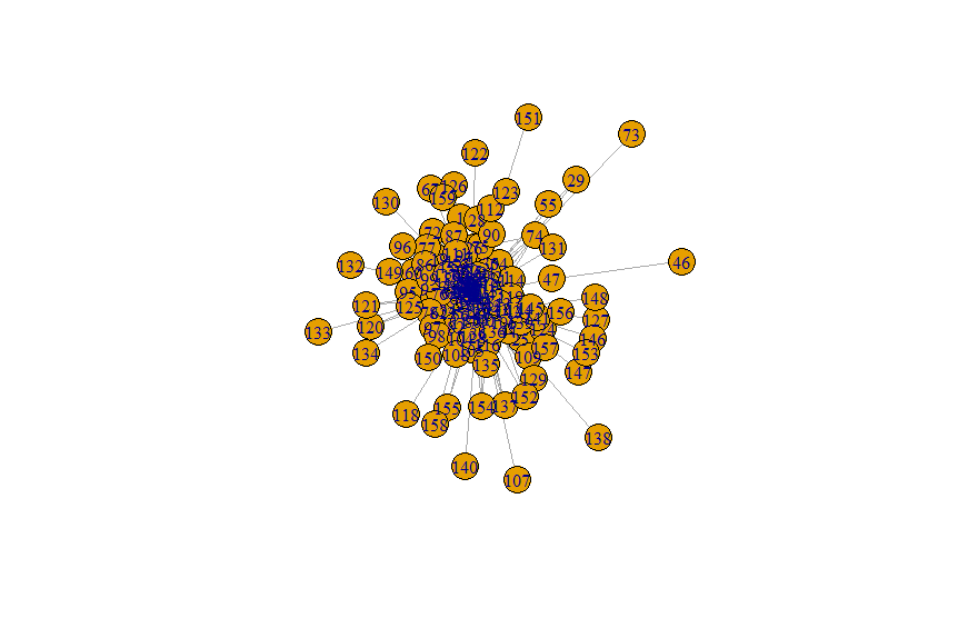
> # 플로팅하기
> plot(od_line_sln@g, edge.width = E(od_line_sln@g)$weight/100)
>
> ## 모형별 모듈성 비교
> # 모듈성 : 그룹 안의 링크가 그룹 밖과 연결된 링크보다 더 많다는 정도를 알려주는 지표
> # cluster-spinglass 알고리즘
> modulos <- cluster_spinglass(od_line_sln@g)
> modularity(modulos)
[1] 0.007664102
> # walktrap 알고리즘
> modulos <- walktrap.community(od_line_sln@g)
> modularity(modulos)
[1] 0.2267285
> # multilevel 알고리즘
> modulos <- multilevel.community(od_line_sln@g)
> modularity(modulos)
[1] 0.2397323
> # multilevel의 성능이 가장 우수한 것으로 나타났다.
>
> ## 지도 시각화
> # 꼭지점 좌푯값 추출
> l_out <- cbind(od_line_sln@g$x, od_line_sln@g$y)
> # 화면 분할
> par(mfrow=c(1,2))
> # 사람들 이동에 대한 욕구선 그리기
> plot(admin, lwd = 1, border = "grey", main = "Desire Line", xlim = c(126.93, 127.16), ylim = c(37.1, 37.3))
> plot(od_line, lwd = (od_line$총이용객수)/300, col = "orange", rescale = T, add = T)
Warning message:
In plot.sf(od_line, lwd = (od_line$총이용객수)/300, col = "orange", :
ignoring all but the first attribute
> # 욕구선 기반 커뮤니티 탐지
> plot(admin, lwd = 1, border = "grey", main = "Community Detection", xlim = c(126.93, 127.16), ylim = c(37.1, 37.3))
> plot.igraph(od_line_sln@g, vertex.label = NA,
+ vertex.size = 0.05*igraph::degree(od_line_sln@g),
+ vertex.color = adjustcolor("blue", alpha.f = .4),
+ edge.width = edge_attr(od_line_sln@g)$weight/1000,
+ edge.color = "orange",
+ edge.curved = 0.3,
+ layout = l_out,
+ mark.groups = modulos,
+ mark.border = "NA",
+ rescale = F, add = T
+ )

>
>
> ## 7 교통 흐름 분석 2 : 비통근 시간대
>
>
> # Step 1 : 비통근 시간대 교통 흐름 분석
>
> ## 비통근 시간대 데이터 필터링
> # 데이터 불러오기
> setwd(dirname(rstudioapi::getSourceEditorContext()$path))
> load("./01_save/04_002_trip_chain.rdata")
> load("./01_save/04_001_sta_pnt.rdata")
> load("./01_save/01_002_fishnet.rdata")
> load("./01_save/01_001_admin.rdata")
> # 비통근 통행 필터링 (10~16시)
> library(dplyr)
> trip_cmt <- trip_chain[grep("10|11|12|13|14|15|16", trip_chain$start_hour),]
> # trip_cmt 번호 다시 매기기
> rownames(trip_cmt) <- 1:nrow(trip_cmt)
> save(trip_cmt, file = "./01_save/07_001_trip_cmt.rdata")
> # trip_cmt에서 필요한 정보만 추출하기
> keeps <- c("id.x", "id.y", "승차역ID1", "최종하차역ID", "총이용객수", "환승횟수")
> grid_chain <- trip_cmt[keeps]
> head(grid_chain)
id.x id.y 승차역ID1 최종하차역ID 총이용객수 환승횟수
1 2630 3185 4100049 4100017 1 1
2 2630 3185 4100049 4100017 1 1
3 2630 3185 4100049 4100017 2 1
4 2541 3185 4170974 4100017 1 1
5 2632 3185 4197604 4100017 1 2
6 2630 3185 4100049 4100017 1 1
> save(grid_chain, file = "./01_save/07_001_grid_chain.rdata")
> rm("trip_chain"); rm("keeps")
>
> ## 집계구 간 이동만 남기기(집계구 내 이동 지우기)
> library(stplanr)
> od_intra <- filter(grid_chain, id.x != id.y)
> # 그리드 간(intra) 이동별 총이용객수, 환승횟수 집계하기
> od_intra2 <- od_intra %>%
+ group_by(id.x, id.y) %>%
+ summarise_each(funs(sum)) %>%
+ dplyr::select(id.x, id.y, 총이용객수, 환승횟수)
> # 평균 환승횟수 계산
> od_intra2$평균환승 <- round((od_intra2$환승횟수 / od_intra2$총이용객수), 1)
> # 컬럼 이름 정리하기
> colnames(od_intra2) <- c("id.x", "id.y", "총이용객수", "환승횟수", "평균환승")
> head(od_intra2)
# A tibble: 6 x 5
# Groups: id.x [3]
id.x id.y 총이용객수 환승횟수 평균환승
<int> <int> <dbl> <dbl> <dbl>
1 1348 2822 1 3 3
2 1349 2541 16 24 1.5
3 1349 2545 16 16 1
4 1349 2633 8 8 1
5 1439 2544 2 6 3
6 1439 2716 2 4 2
>
> ## 시각화 위하여 공간 데이터 형식(OD2LINE)으로 변경
> # 공간 데이터 형식(OD2LINE) 만들기
> od_line <- od2line(od_intra2, as(fishnet, "sf"))
Creating centroids representing desire line start and end points.
> # 저장
> save(od_line, file = "./01_save/07_003_od_line.rdata")
> # 총이용객수 시각화
> library(tmap)
> qtm("Hwaseong")
Switching to view mode. Run tmap_mode("plot") or simply ttm() to switch back to plot mode.
> qtm("Hwaseong") +
+ tm_basemap("OpenStreetMap") +
+ qtm(subset(od_line, od_line$총이용객수 > 30), lines.col = "grey", lines.lwd = .3) +
+ qtm(subset(od_line, od_line$총이용객수 > 100), lines.col = "blue", lines.alpha = .4, lines.lwd = 1) +
+ qtm(subset(od_line, od_line$총이용객수 > 40), lines.col = "orange", lines.alpha = .6, lines.lwd = 2) +
+ qtm(subset(od_line, od_line$총이용객수 > 1000), lines.col = "red", lines.alpha = .8, lines.lwd = 4)
Warning message:
qtm called without shape objects cannot be stacked
> # 평균환승 시각화
> qtm("Hwaseong")
> qtm("Hwaseong") +
+ tm_basemap("OpenStreetMap") +
+ qtm(subset(od_line, od_line$평균환승 >= 0 & od_line$평균환승 < 2), lines.col = "grey", lines.lwd = .3) +
+ qtm(subset(od_line, od_line$평균환승 >= 2 & od_line$평균환승 < 3), lines.col = "blue", lines.alpha = .4, lines.lwd = 1) +
+ qtm(subset(od_line, od_line$평균환승 >= 3 & od_line$평균환승 < 9), lines.col = "red", lines.alpha = .4, lines.lwd = 2)
Warning message:
qtm called without shape objects cannot be stacked
>
>
> # Step 2 : 비통근 시간대 커뮤니티 탐지
>
> ## 네트워크 속성 변환 (Spatial_data_frame => Spatial_Network)
> library(stplanr)
> # 네트워크 데이터로 변환
> od_line_sln <- SpatialLinesNetwork(od_line)
> # g, nb 등 확인
> head(od_line_sln@nb, 2)
[[1]]
[1] 1
[[2]]
[1] 1 91 137 161 206 240 264 374 482 589 664 697 749 782 819 870 895 1115 1128 1191 1192 1193 1194
[24] 1195 1196 1197 1198 1199 1200 1201 1202 1203 1204 1205 1206
> head(od_line_sln@g, 2)
2 x 147 sparse Matrix of class "dgCMatrix"
[1,] . 17879.05 . . . . . . . . . . . . . . . . . . . . .
[2,] 17879.05 . . 11089.28 6902.904 . . 7554.161 . . . . 2091.814 . 5686.386 . . 7040.85 4787.671 1771.911 . . .
[1,] . . . . . . . . . . . . . . . . . . . . . . . . . . . . . . . .
[2,] 7107.799 . 6274.847 . . 4264.899 7427.457 . 7832.155 . . . . . . . . . . . . . . . . 17283.63 5761.534 . . . . .
[1,] . . . . . . . . . . . . . . . . . . . . . . . . . . . . . .
[2,] 12730.02 . . . . . 2843.339 . . . . . . . 10163.03 . 9574.822 . . . . . . . . 9950.407 3335.853 2223.902 . 8954.89
[1,] . . . . . . . . . . . . . . . . . . . . . . . . . . . . . . . . . . . . . . . . . . . .
[2,] 7982.611 . . 18214.5 . . . . . . . . . 4184.225 . . . . 4866.374 . . . . . . . . . . . . . . . . . . . . . . . . .
[1,] . . . . . . . . . . . . . . . . . .
[2,] . . . 15964.86 . . . . . . . . . . . . . .
> # 네트워크 가중치 부여하기
> library(igraph)
> E(od_line_sln@g)$weight <- od_line$총이용객수
> # 엣지 속성 보기
> edge_attr(od_line_sln@g)$weight
[1] 1 16 16 8 2 2 1 1 8 2 8 16 6 2 2 3 2 1 8 8 5 12 1
[24] 2 4 2 12 8 2 20 16 1 1 1 2 6 12 8 2 2 1 4 1 1 4 2
[47] 8 8 8 10 1 2 6 1 8 13 6 5 1 5 2 6 5 3 90 2 2 3 1
...
[990] 2 2 1 6 9 3 2 1 1 1 1
[ reached getOption("max.print") -- omitted 442 entries ]
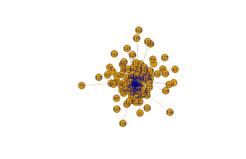
> # 플로팅하기
> plot(od_line_sln@g, edge.width = E(od_line_sln@g)$weight/100)
>
> ## 모형별 모듈성 비교
> # cluster-spinglass 알고리즘
> modulos <- cluster_spinglass(od_line_sln@g)
> modularity(modulos)
[1] 0.01026044
> # walktrap 알고리즘
> modulos <- walktrap.community(od_line_sln@g)
> modularity(modulos)
[1] 0.2064825
> # multilevel 알고리즘
> modulos <- multilevel.community(od_line_sln@g)
> modularity(modulos)
[1] 0.2305334
> # multilevel의 성능이 가장 우수한 것으로 나타났다.
>
> ## 지도 시각화
> # 꼭지점 좌푯값 추출
> l_out <- cbind(od_line_sln@g$x, od_line_sln@g$y)
> # 화면 분할
> par(mfrow=c(1,2))
> # 사람들 이동에 대한 욕구선 그리기
> plot(admin, lwd = 1, border = "grey", main = "Desire Line", xlim = c(126.93, 127.16), ylim = c(37.1, 37.3))
> plot(od_line, lwd = (od_line$총이용객수)/300, col = "orange", rescale = T, add = T)
Warning message:
In plot.sf(od_line, lwd = (od_line$총이용객수)/300, col = "orange", :
ignoring all but the first attribute
> # 욕구선 기반 커뮤니티 탐지
> plot(admin, lwd = 1, border = "grey", main = "Community Detection", xlim = c(126.93, 127.16), ylim = c(37.1, 37.3))
> plot.igraph(od_line_sln@g, vertex.label = NA,
+ vertex.size = 0.05*igraph::degree(od_line_sln@g),
+ vertex.color = adjustcolor("blue", alpha.f = .4),
+ edge.width = edge_attr(od_line_sln@g)$weight/1000,
+ edge.color = "orange",
+ edge.curved = 0.3,
+ layout = l_out,
+ mark.groups = modulos,
+ mark.border = "NA",
+ rescale = F, add = T
+ )

출처 : 김철민, ⌜공공데이터로 배우는 R 데이터분석 with 샤이니⌟, 이지스퍼블리싱, 2022
'데이터분석 > R' 카테고리의 다른 글
| [R 통계분석] 기술통계학 (0) | 2022.08.09 |
|---|---|
| [R 데이터분석 with 샤이니] 교통 카드 데이터 분석 사례 04 - 종합 분석 (0) | 2022.08.06 |
| [R 데이터분석 with 샤이니] 교통 카드 데이터 분석 사례 02 - 기초 분석 (0) | 2022.07.30 |
| [R 데이터분석 with 샤이니] 교통 카드 데이터 분석 사례 01 - 데이터 전처리 (0) | 2022.07.30 |
| [R 데이터분석 with 샤이니] 커피 전문점 접근성 분석 (Shiny) (0) | 2022.07.28 |


