Section 01. 모집단이 두 개
> # 테스트 데이터 준비
> install.packages("PairedData")
> library(PairedData)
> data(Anorexia)
> Anorexia
Prior Post
1 83.8 95.2
2 83.3 94.3
3 86.0 91.5
4 82.5 91.9
5 86.7 100.3
...
17 87.3 98.0
> write.csv(Anorexia, "./data/01.anorexia.csv", row.names=FALSE)
>
> # 남자 아이와 여자 아이의 체중 (독립적인 두 집단)
>
> data <- read.table("./data/chapter7.txt", header=T)
>
> par(mar=c(2, 1, 1, 1))
> hist(data$weight[data$gender==1], xlim=c(1500, 4500), ylim=c(0, 12), col="green", border=NA, main="", xlab="", ylab="", axes=F)
> hist(data$weight[data$gender==2], density=10, angle=45, add=TRUE, col="orange")
> abline(v = mean(data$weight[data$gender==1]), lty=3, lwd=1.5, col="green")
> abline(v = mean(data$weight[data$gender==2]), lty=1, lwd=1.5, col="orange")
> legends = c("여자아이", "남자아이")
> legend("topright", legend=legends, fill=c("green", "orange"), density=c(NA, 20))

>
> # 분산의 동일성 여부에 따른 차이
>
> x <- seq(-3, 3, by=0.01)
> y <- dnorm(x)
>
> plot(x, y, type="l", xlim=c(-3, 3.5), ylim=c(0, 0.5), axes=FALSE)
> axis(1)
> lines(c(0, 0), c(0, max(y)), lty=3)
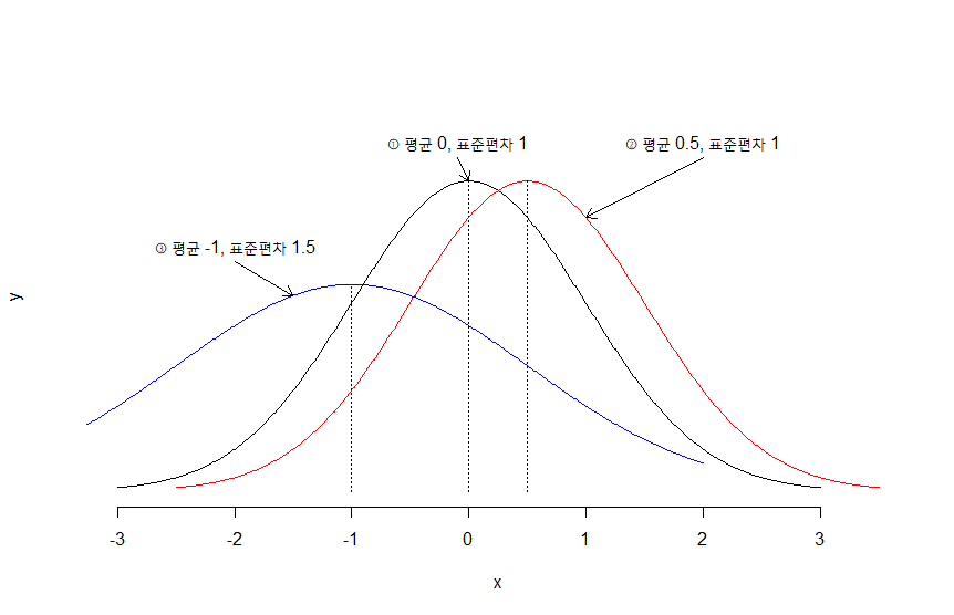
> text(-0.1, max(y)+0.05, "① 평균 0, 표준편차 1")
> arrows(-0.1, max(y)+0.03, 0, max(y), length=0.1)
>
> y2 <- dnorm(x+0.5, mean=0.5)
> lines(x+0.5, y2, col="red")
> lines(c(0.5, 0.5), c(0, max(y2)), lty=3)
> text(2, max(y2)+0.05, "② 평균 0.5, 표준편차 1")
> arrows(2, max(y2)+0.03, 1, dnorm(1, mean=0.5), length=0.1)
>
> y3 <- dnorm(x-1, mean=-1, sd=1.5)
> lines(x-1, y3, col="blue")
> lines(c(-1, -1), c(0, max(y3)), lty=3)
> text(-2, max(y3)+0.05, "③ 평균 -1, 표준편차 1.5")
> arrows(-2, max(y3)+0.03, -1.5, dnorm(-1.5, mean=-1, sd=1.5), length=0.1)
>
> # ①과 ③처럼 모분산이 동일하지 않을 경우에는 평균 중심으로 분포할 확률이 서로 다르다.
> # 따라서 이 부분을 보정하기 위해 검정통계량에 따르는 t-분포의 자유도를 표본의 개수를 통해 구하지 않고 다른 방법으로 구하여 비교할 수 있다.
> # 모분상의 동일성 여부는 표본으로 추출된 자료를 통해 가설검정의 단계를 거쳐 확인한다.
>
> ## 01) 서로 독립인 두 집단에서의 평균 차이 검정
>
> # 남아 신생아와 여아 신생아의 몸무게
>
> # 등분산성 검정
> data <- read.table("./data/chapter7.txt", header=T)
> var.test(data$weight ~ data$gender)
F test to compare two variances
data: data$weight by data$gender
F = 2.1771, num df = 17, denom df = 25, p-value = 0.07526
alternative hypothesis: true ratio of variances is not equal to 1
95 percent confidence interval:
0.9225552 5.5481739
sample estimates:
ratio of variances
2.177104
> (cu <- qf(0.975, df1 = 17, df2 = 25))
[1] 2.359863
> # 유의확률이 0.07526으로 유의수준 0.05보다 크므로 대립가설을 기각한다.
> # 즉 남아 신생아와 여아 신생아의 몸무게의 분산은 서로 동일하다고 할 수 있다.
> # 평균 차이 검정을 실시한다.
>
> # 서로 독립인 두 집단의 평균 비교
> t.test(data$weight ~ data$gender,
+ mu = 0, alternative = "less", var.equal = TRUE)
Two Sample t-test
data: data$weight by data$gender
t = -1.5229, df = 42, p-value = 0.06764
alternative hypothesis: true difference in means between group 1 and group 2 is less than 0
95 percent confidence interval:
-Inf 25.37242
sample estimates:
mean in group 1 mean in group 2
3132.444 3375.308
> # 유의확률이 0.06784로 유의수준 0.05보다 크므로 대립가설을 기각한다.
> # 즉 남아 몸무게의 평균이 여아 몸무게의 평균보다 크지 않은 것으로 판단된다.
>
> ## 02) 서로 대응인 두 집단에서의 평균 차이 검정
>
> # 식욕부진증 치료요법의 효과 검정
>
> data <- read.csv("./data/01.anorexia.csv", header=T)
> str( data )
'data.frame': 17 obs. of 2 variables:
$ Prior: num 83.8 83.3 86 82.5 86.7 79.6 76.9 94.2 73.4 80.5 ...
$ Post : num 95.2 94.3 91.5 91.9 100.3 ...
>
> # 표본의 크기
> n <- length(data$Prior - data$Post)
> # 표본 평균
> m <- mean(data$Prior - data$Post)
> # 표준편차
> s <- sd(data$Prior - data$Post)
> # 대응별 차이의 평균
> m <- mean(data$Prior - data$Post)
> # 대응별 차이의 편차
> s <- sd(data$Prior - data$Post)
> # 검정통계량 계산
> (t.t <- m/(s/sqrt(n)))
[1] -4.184908
>
> # 대응인 두 집단의 평균 차이 검정
> t.test(data$Prior, data$Post, paired = T, alternative = "less")
Paired t-test
data: data$Prior and data$Post
t = -4.1849, df = 16, p-value = 0.0003501
alternative hypothesis: true mean difference is less than 0
95 percent confidence interval:
-Inf -4.233975
sample estimates:
mean difference
-7.264706
> # 유의확률이 0.0003501로 유의수준 0.05보다 작으므로 대립가설을 채택한다.
> # 즉 식욕부진증 치료요법은 효과가 있는 것으로 판단된다.
Section 02. 모집단이 세 개 이상
>
> # 일원분산분석 모형에 따른 집단별 자료의 분포
>
> set.seed(2)
> grp1 <- rnorm(20, mean=-1)
> grp2 <- rnorm(20, mean=0.5)
> grp3 <- rnorm(20, mean=1)
>
> d <- data.frame(grp=rep(1:3, each=20), val=c(grp1, grp2, grp3))
>
> par(mar=c(1, 1, 1, 1))
> plot(val~grp, data=d, pch=20, col="red", xlim=c(1, 3.5), ylim=c(-4.2, 4), axes=F, xlab="", ylab="")
>
> text(1.2, -4, "처리 1")
> text(2.2, -3, "처리 2")
> text(3.2, -2, "처리 3")
>
> abline(h=mean(d$val), lwd=2, col="red")
> arrows(1.5, 1.9, 1.5, mean(d$val), length=0.1)
> text(1.5, 2.2, expression(bar(y[..]) ), cex=1.5)
>
> lines(c(1, 1), c(-4, 2), lty=2, col="blue")
> lines(c(2, 2), c(-2.5, 3.5), lty=2, col="blue")
> lines(c(3, 3), c(-2, 4), lty=2, col="blue")
>
> y1 <- seq(-4, 2, by=0.01)
> x1 <- 1+dnorm(y1, mean=-1)
> lines(x1, y1, lty=3, lwd=1.5, col="blue")
> lines(c(1, max(x1)), c(-1, -1), lty=2)
> arrows(1.5, -3, 1.3, -2, length=0.05)
> text(1.5, -3.2, expression(N(mu[1], sigma^2) ))
>
> y2 <- seq(-2.5, 3.5, by=0.01)
> x2 <- 2+dnorm(y2, mean=0.5)
> lines(x2, y2, lty=3, lwd=1.5, col="blue")
> lines(c(2, max(x2)), c(0.5, 0.5), lty=2)
> arrows(2.4, 1.8, 2.3, 1.3, length=0.05)
> text(2.5, 2.2, expression(N(mu[2], sigma^2) ))
>
> y3 <- seq(-2, 4, by=0.01)
> x3 <- 3+dnorm(y3, mean=1)
> lines(x3, y3, lty=3, lwd=1.5, col="blue")
> lines(c(3, max(x3)), c(1, 1), lty=2)
> arrows(3.4, 2.8, 3.3, 2, length=0.05)
> text(3.4, 3.2, expression(N(mu[3], sigma^2) ))

>
> ## 03) 세 집단 이상에서의 평균 차이 검정
>
> # 각 지역규모별 나이의 평균 비교 검증
>
> ad <- read.csv("./data/age.data.csv", header=T)
> str(ad)
'data.frame': 150 obs. of 4 variables:
$ scale: int 1 1 1 1 1 1 1 1 1 1 ...
$ sex : int 2 2 2 1 1 2 1 2 2 2 ...
$ score: int 8 5 7 4 5 3 3 7 9 4 ...
$ age : int 56 33 49 53 74 42 51 59 25 57 ...
> summary(ad)
scale sex score age
Min. :1 Min. :1.000 Min. : 1.00 Min. :14.00
1st Qu.:1 1st Qu.:1.000 1st Qu.: 4.00 1st Qu.:38.00
Median :2 Median :2.000 Median : 6.00 Median :46.00
Mean :2 Mean :1.507 Mean : 8.22 Mean :46.51
3rd Qu.:3 3rd Qu.:2.000 3rd Qu.: 7.00 3rd Qu.:56.00
Max. :3 Max. :2.000 Max. :99.00 Max. :89.00
> ad$score <- ifelse(ad$score==99, NA, ad$score)
> ad$scale <- factor(ad$scale)
> ad$sex <- factor(ad$sex)
> str(ad)
'data.frame': 150 obs. of 4 variables:
$ scale: Factor w/ 3 levels "1","2","3": 1 1 1 1 1 1 1 1 1 1 ...
$ sex : Factor w/ 2 levels "1","2": 2 2 2 1 1 2 1 2 2 2 ...
$ score: int 8 5 7 4 5 3 3 7 9 4 ...
$ age : int 56 33 49 53 74 42 51 59 25 57 ...
>
> # 분석을 위한 통계량 계산과 오차제곱합 구하기
>
> y1 <- ad$age[ad$scale == "1"]
> y2 <- ad$age[ad$scale == "2"]
> y3 <- ad$age[ad$scale == "3"]
>
> y1.mean <- mean(y1)
> y2.mean <- mean(y2)
> y3.mean <- mean(y3)
>
> # 각 처리내 편차제곱합
> sse.1 <- sum( (y1 - y1.mean)^2 )
> sse.2 <- sum( (y2 - y2.mean)^2 )
> sse.3 <- sum( (y3 - y3.mean)^2 )
>
> # 오차제곱합
> (sse <- sse.1 + sse.2 + sse.3)
[1] 30139.38
> # 자유도
> (dfe <- (length(y1)-1) + (length(y2)-1) + (length(y3)-1))
[1] 147
>
> y <- mean(ad$age)
>
> # 각 처리간 편차제곱합
> sst.1 <- length(y1) * sum((y1.mean - y)^2)
> sst.2 <- length(y2) * sum((y2.mean - y)^2)
> sst.3 <- length(y3) * sum((y3.mean - y)^2)
>
> # 처리제곱합
> (sst <- sst.1 + sst.2 + sst.3)
[1] 150.0933
> # 자유도
> (dft <- length(levels(ad$scale)) - 1)
[1] 2
>
> # 전체제곱합
> (tsq <- sum((ad$age - y)^2))
[1] 30289.47
> # 분해된 제곱합의 합
> (ss <- sst + sse)
[1] 30289.47
> # 전체제곱합이 오차제곱합과 처리제곱합으로 분해되었음을 확인할 수 있다.
>
> # 처리 평균 제곱합
> mst <- sst / dft
> # 오차 평균제곱합
> mse <- sse / dfe
> # 검정통계량 구하기
> (f.t <- mst / mse)
[1] 0.3660281
>
> # 기각역을 위한 임계값 구하기
> alpha <- 0.05
> (tol <- qf(1-alpha, dft, dfe))
[1] 3.057621
>
> # 유의확률 구하기
> (p.value <- 1 - pf(f.t, dft, dfe))
[1] 0.6941136
>
> # lm() 함수와 anova() 함수를 사용한 분석
> ow <- lm(age~scale, data=ad)
> anova(ow)
Analysis of Variance Table
Response: age
Df Sum Sq Mean Sq F value Pr(>F)
scale 2 150.1 75.047 0.366 0.6941
Residuals 147 30139.4 205.030
>
> # 유의확률이 0.6941로 유의수준 0.05보다 크므로 대립가설을 기각한다.
> # 즉 각 지역규모별 나이의 평균값은 차이가 없다고 할 수 있다.
출처 : 이윤환, ⌜제대로 알고 쓰는 R 통계분석⌟, 한빛아카데미, 2020
'데이터분석 > R' 카테고리의 다른 글
| [R 통계분석] 상관과 회귀 (0) | 2022.08.27 |
|---|---|
| [R 통계분석] 범주형 자료분석 (0) | 2022.08.19 |
| [R 통계분석] 가설검정 (0) | 2022.08.12 |
| [R 통계분석] 추정 (0) | 2022.08.11 |
| [R 통계분석] 표본분포 (0) | 2022.08.10 |


