> ## Chapter5-2. 병아리의 무게를 예측할 수 있을까? (회귀분석)
>
> # 단순선형 회귀분석 실시
> w_lm <- lm(weight ~ egg_weight, data = w_n)
> # 회귀모델 결과 확인
> summary(w_lm)
Call:
lm(formula = weight ~ egg_weight, data = w_n)
Residuals:
Min 1Q Median 3Q Max
-3.0177 -1.7148 0.1394 1.8080 2.9594
Coefficients:
Estimate Std. Error t value Pr(>|t|)
(Intercept) -14.5475 8.7055 -1.671 0.106
egg_weight 2.3371 0.1336 17.493 <2e-16 ***
---
Signif. codes: 0 ‘***’ 0.001 ‘**’ 0.01 ‘*’ 0.05 ‘.’ 0.1 ‘ ’ 1
Residual standard error: 2.055 on 28 degrees of freedom
Multiple R-squared: 0.9162, Adjusted R-squared: 0.9132
F-statistic: 306 on 1 and 28 DF, p-value: < 2.2e-16
>
> # 산점도에 회귀직선을 표시해 모델이 데이터를 잘 대표하는지 확인
> plot(w_n$egg_weight, w_n$weight) # 산점도 그리기
> lines(w_n$egg_weight, w_lm$fitted.values, col = "blue") # 회귀직선 추가
> text(x = 66, y = 132, label = 'Y = 2.3371X - 14.5475') # 회귀직선 라벨로 표시

>
> names(w_lm) # w_lm 변수에 어떤 항목들이 있는지 확인
[1] "coefficients" "residuals" "effects" "rank" "fitted.values" "assign" "qr"
[8] "df.residual" "xlevels" "call" "terms" "model"
>
> w_lm$coefficients
(Intercept) egg_weight
-14.547529 2.337136
> w_lm$model
weight egg_weight
1 140 65
2 128 62
3 140 65
4 135 65
5 145 69
...
30 135 63
>
> hist(w_lm$residuals, col = "skyblue", xlab = "residuals",
+ main = "병아리 무게 잔차 히스토그램")
> # 잔차가 0 근처에 주로 분포해 세로가 긴 종 모양의 히스토그램이 나왔으면 좋겠지만 잔차가 다양하게 분포한 형태로 나왔다.
> # 잔차를 더 줄이기 위해 독립변수를 더 늘리는 방법을 생각해 볼 수 있다.
>
>
> # 다중회귀분석 실시
> w_mlm <- lm(weight ~ egg_weight + movement + food, data = w_n)
> summary(w_mlm)
Call:
lm(formula = weight ~ egg_weight + movement + food, data = w_n)
Residuals:
Min 1Q Median 3Q Max
-3.2037 -1.3079 0.1826 1.2572 2.3647
Coefficients:
Estimate Std. Error t value Pr(>|t|)
(Intercept) 2.974830 8.587203 0.346 0.731811
egg_weight 1.776350 0.194845 9.117 1.4e-09 ***
movement -0.008674 0.016631 -0.522 0.606417
food 1.584729 0.404757 3.915 0.000583 ***
---
Signif. codes: 0 ‘***’ 0.001 ‘**’ 0.01 ‘*’ 0.05 ‘.’ 0.1 ‘ ’ 1
Residual standard error: 1.681 on 26 degrees of freedom
Multiple R-squared: 0.9479, Adjusted R-squared: 0.9419
F-statistic: 157.7 on 3 and 26 DF, p-value: < 2.2e-16
>
> # p값이 높은 movement 변수를 제외한 열만 다시 회귀분석 실시
> w_mlm2 <- lm(weight ~ egg_weight + food, data = w_n)
> summary(w_mlm2)
Call:
lm(formula = weight ~ egg_weight + food, data = w_n)
Residuals:
Min 1Q Median 3Q Max
-3.0231 -1.2124 0.2445 1.3607 2.2352
Coefficients:
Estimate Std. Error t value Pr(>|t|)
(Intercept) 3.6638 8.3698 0.438 0.665052
egg_weight 1.7453 0.1830 9.536 3.89e-10 ***
food 1.5955 0.3987 4.001 0.000441 ***
---
Signif. codes: 0 ‘***’ 0.001 ‘**’ 0.01 ‘*’ 0.05 ‘.’ 0.1 ‘ ’ 1
Residual standard error: 1.658 on 27 degrees of freedom
Multiple R-squared: 0.9474, Adjusted R-squared: 0.9435
F-statistic: 243 on 2 and 27 DF, p-value: < 2.2e-16
>
> # 다중공선성(Multicollinearity) 확인을 위한 패키지
> library(car)
필요한 패키지를 로딩중입니다: carData
경고메시지(들):
1: 패키지 ‘car’는 R 버전 4.0.3에서 작성되었습니다
2: 패키지 ‘carData’는 R 버전 4.0.3에서 작성되었습니다
>
> # 분산팽창요인(Variation Inflation Factor, VIF)
> # 10이상이면 문제있다고 보고, 30보다 크면 심각
> vif(w_mlm2)
egg_weight food
2.882685 2.882685
>
> # 잔차 히스토그램
> hist(w_mlm2$residuals, col = "skyblue", xlab = "residuals",
+ main = "병아리 무게 잔차 히스토그램(다중 회귀)")

> # 단순 선형 회귀분석 결과 대비 잔차의 분포가 중심이 긴 종 모양 형태에 가까워졌음을 확인할 수 있다.
>
> # (참고)후진소거법을 적용해 자동으로 실행
> step_mlm <- step(w_mlm, direction = "backward")
Start: AIC=34.88
weight ~ egg_weight + movement + food
Df Sum of Sq RSS AIC
- movement 1 0.769 74.262 33.192
<none> 73.494 34.880
- food 1 43.331 116.825 46.784
- egg_weight 1 234.940 308.433 75.909
Step: AIC=33.19
weight ~ egg_weight + food
Df Sum of Sq RSS AIC
<none> 74.26 33.192
- food 1 44.034 118.30 45.160
- egg_weight 1 250.123 324.39 75.422
>
> # (참고)회귀분석 결과 그래프로 확인
> plot(w_mlm2)
다음 플랏을 보기 위해서는 <Return>키를 치세요

다음 플랏을 보기 위해서는 <Return>키를 치세요

다음 플랏을 보기 위해서는 <Return>키를 치세요

다음 플랏을 보기 위해서는 <Return>키를 치세요

>
>
> # 비선형 회귀분석용 두번째 데이터셋 불러오기
> w2 <- read.csv("ch5-2.csv", header = TRUE)
> head(w2)
day weight
1 1 43
2 2 55
3 3 69
4 4 86
5 5 104
6 6 124
> str(w2)
'data.frame': 70 obs. of 2 variables:
$ day : int 1 2 3 4 5 6 7 8 9 10 ...
$ weight: int 43 55 69 86 104 124 147 172 200 229 ...
>
> plot(w2) # 데이터 형태 산점도로 확인

>
> # 성장기간에 따른 병아리 무게 변화 선형 회귀분석 실시
> w2_lm <- lm(weight ~ day, data = w2)
> summary(w2_lm)
Call:
lm(formula = weight ~ day, data = w2)
Residuals:
Min 1Q Median 3Q Max
-416.65 -138.42 -12.21 151.32 282.05
Coefficients:
Estimate Std. Error t value Pr(>|t|)
(Intercept) -295.867 41.102 -7.198 6.22e-10 ***
day 56.822 1.006 56.470 < 2e-16 ***
---
Signif. codes: 0 ‘***’ 0.001 ‘**’ 0.01 ‘*’ 0.05 ‘.’ 0.1 ‘ ’ 1
Residual standard error: 170.1 on 68 degrees of freedom
Multiple R-squared: 0.9791, Adjusted R-squared: 0.9788
F-statistic: 3189 on 1 and 68 DF, p-value: < 2.2e-16
>
> # 산점도 위에 회귀직선 표시
> lines(w2$day, w2_lm$fitted.values, col = "blue")

> # 산점도와 직선을 같이 표시하고 보니 3차 함수의 그래프와 유사함을 발견할 수 있다.
>
> # 성장기간에 따른 병아리 무게 변화 비선형 회귀분석 실시
> w2_lm2 <- lm(weight ~ I(day^3) + I(day^2) + day, data = w2)
> summary(w2_lm2)
Call:
lm(formula = weight ~ I(day^3) + I(day^2) + day, data = w2)
Residuals:
Min 1Q Median 3Q Max
-61.315 -22.821 -1.336 22.511 48.772
Coefficients:
Estimate Std. Error t value Pr(>|t|)
(Intercept) 1.170e+02 1.348e+01 8.683 1.59e-12 ***
I(day^3) -2.529e-02 4.929e-04 -51.312 < 2e-16 ***
I(day^2) 2.624e+00 5.321e-02 49.314 < 2e-16 ***
day -1.530e+01 1.632e+00 -9.373 9.51e-14 ***
---
Signif. codes: 0 ‘***’ 0.001 ‘**’ 0.01 ‘*’ 0.05 ‘.’ 0.1 ‘ ’ 1
Residual standard error: 26.69 on 66 degrees of freedom
Multiple R-squared: 0.9995, Adjusted R-squared: 0.9995
F-statistic: 4.407e+04 on 3 and 66 DF, p-value: < 2.2e-16
>
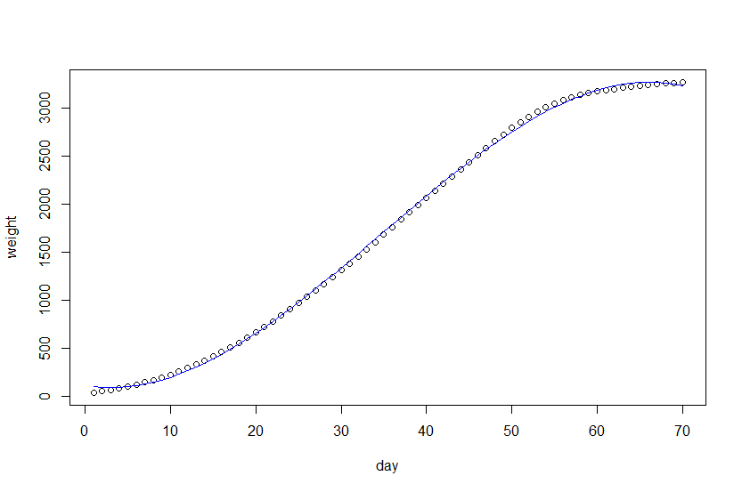
> plot(w2)
> # 산점도 위에 회귀곡선 표시
> lines(w2$day, w2_lm2$fitted.values, col = "blue")
>
> # w2_lm2 회귀분석 결과에서 계수 확인
> w2_lm2$coefficients
(Intercept) I(day^3) I(day^2) day
117.01408122 -0.02529014 2.62414840 -15.29781677
>
> # 산점도 위에 수식 표시
> text(25, 3000, "weight = -0.025*day^3 + 2.624*day^2 - 15.298*day + 117.014")

출처 : 현장에서 바로 써먹는 데이터 분석 with R
'데이터분석 > R' 카테고리의 다른 글
| [현장에서 바로 써먹는...] 분류분석 (0) | 2022.04.09 |
|---|---|
| [현장에서 바로 써먹는...] 로지스틱 회귀 (0) | 2022.04.09 |
| [현장에서 바로 써먹는...] 상관분석 (0) | 2022.04.05 |
| [현장에서 바로 써먹는...] 가설검정 (0) | 2022.04.02 |
| [현장에서 바로 써먹는...] 정규분포와 중심극한정리 (0) | 2022.04.02 |


