> ## Chapter 6-2. 병아리 품종을 구분할 수 있을까? (분류 알고리즘)
>
>
> # Naive Bayes
> library(e1071)
>
> c_train <- read.csv("ch6-2_train.csv", header = TRUE)
> c_test <- read.csv("ch6-2_test.csv", header = TRUE)
> str(c_train)
'data.frame': 240 obs. of 4 variables:
$ wing_length: int 238 236 256 240 246 233 235 241 232 234 ...
$ tail_length: int 63 67 65 63 65 65 66 66 64 64 ...
$ comb_height: int 34 30 34 35 30 30 30 35 31 30 ...
$ breeds : chr "a" "a" "a" "a" ...
> str(c_test)
'data.frame': 60 obs. of 4 variables:
$ wing_length: int 258 260 251 248 254 230 248 250 235 241 ...
$ tail_length: int 67 64 63 63 62 64 65 65 62 67 ...
$ comb_height: int 32 34 31 30 32 33 35 33 35 30 ...
$ breeds : chr "a" "a" "a" "a" ...
> c_train$breeds <- as.factor(c_train$breeds)
> c_test$breeds <- as.factor(c_test$breeds)
> str(c_test)
'data.frame': 60 obs. of 4 variables:
$ wing_length: int 258 260 251 248 254 230 248 250 235 241 ...
$ tail_length: int 67 64 63 63 62 64 65 65 62 67 ...
$ comb_height: int 32 34 31 30 32 33 35 33 35 30 ...
$ breeds : Factor w/ 3 levels "a","b","c": 1 1 1 1 1 1 1 1 1 1 ...
>
> # 병아리 품종을 종속변수로 나머지 변수를 독립변수로한 학습 실시
> c_nb <- naiveBayes(breeds ~., data = c_train)
> c_nb
Naive Bayes Classifier for Discrete Predictors
Call:
naiveBayes.default(x = X, y = Y, laplace = laplace)
A-priori probabilities:
Y
a b c
0.3333333 0.3333333 0.3333333
Conditional probabilities:
wing_length
Y [,1] [,2]
a 244.2250 9.409092
b 223.3375 7.990412
c 240.7625 9.878046
tail_length
Y [,1] [,2]
a 64.5625 1.682702
b 68.2625 1.791285
c 71.4250 1.712020
comb_height
Y [,1] [,2]
a 32.3500 1.765349
b 35.7750 1.806984
c 34.0875 1.647351
> names(c_nb)
[1] "apriori" "tables" "levels" "isnumeric" "call"
>
> # 나이브 베이즈 모델에 테스트용 데이터셋을 이용해 품종 분류 실시
> c_test$pred <- predict(c_nb, newdata = c_test, type = "class")
> head(c_test)
wing_length tail_length comb_height breeds pred
1 258 67 32 a a
2 260 64 34 a a
3 251 63 31 a a
4 248 63 30 a a
5 254 62 32 a a
6 230 64 33 a a
>
> confusionMatrix(c_test$pred, c_test$breeds)
Confusion Matrix and Statistics
Reference
Prediction a b c
a 20 1 0
b 0 17 1
c 0 2 19
Overall Statistics
Accuracy : 0.9333
95% CI : (0.838, 0.9815)
No Information Rate : 0.3333
P-Value [Acc > NIR] : < 2.2e-16
Kappa : 0.9
Mcnemar's Test P-Value : NA
Statistics by Class:
Class: a Class: b Class: c
Sensitivity 1.0000 0.8500 0.9500
Specificity 0.9750 0.9750 0.9500
Pos Pred Value 0.9524 0.9444 0.9048
Neg Pred Value 1.0000 0.9286 0.9744
Prevalence 0.3333 0.3333 0.3333
Detection Rate 0.3333 0.2833 0.3167
Detection Prevalence 0.3500 0.3000 0.3500
Balanced Accuracy 0.9875 0.9125 0.9500
>
>
> # k-NN
>
> library(DMwR2)
>
> c_train <- read.csv("ch6-2_train.csv", header = TRUE)
> c_test <- read.csv("ch6-2_test.csv", header = TRUE)
> c_train$breeds <- as.factor(c_train$breeds)
> c_test$breeds <- as.factor(c_test$breeds)
>
> c_knn3 <- kNN(breeds ~., c_train, c_test, k = 3)
> c_test$pred3 <- c_knn3 # 예측값을 c_test 데이터셋에 pred3열을 만들어서 입력
> head(c_test) # 데이터 확인
wing_length tail_length comb_height breeds pred3
1 258 67 32 a a
2 260 64 34 a a
3 251 63 31 a a
4 248 63 30 a a
5 254 62 32 a a
6 230 64 33 a a
>
> confusionMatrix(c_test$pred3, c_test$breeds)
Confusion Matrix and Statistics
Reference
Prediction a b c
a 19 1 0
b 1 18 1
c 0 1 19
Overall Statistics
Accuracy : 0.9333
95% CI : (0.838, 0.9815)
No Information Rate : 0.3333
P-Value [Acc > NIR] : < 2.2e-16
Kappa : 0.9
Mcnemar's Test P-Value : NA
Statistics by Class:
Class: a Class: b Class: c
Sensitivity 0.9500 0.9000 0.9500
Specificity 0.9750 0.9500 0.9750
Pos Pred Value 0.9500 0.9000 0.9500
Neg Pred Value 0.9750 0.9500 0.9750
Prevalence 0.3333 0.3333 0.3333
Detection Rate 0.3167 0.3000 0.3167
Detection Prevalence 0.3333 0.3333 0.3333
Balanced Accuracy 0.9625 0.9250 0.9625
>
> # c_test 데이터 셋에 pred3열을 만들었기 때문에 1~4열까지만 선택해서 테스트 실시
> c_knn5 <- kNN(breeds ~., c_train, c_test[,1:4], k = 5)
> c_test$pred5 <- c_knn5
> confusionMatrix(c_test$pred5, c_test$breeds)
Confusion Matrix and Statistics
Reference
Prediction a b c
a 20 1 0
b 0 18 1
c 0 1 19
Overall Statistics
Accuracy : 0.95
95% CI : (0.8608, 0.9896)
No Information Rate : 0.3333
P-Value [Acc > NIR] : < 2.2e-16
Kappa : 0.925
Mcnemar's Test P-Value : NA
Statistics by Class:
Class: a Class: b Class: c
Sensitivity 1.0000 0.9000 0.9500
Specificity 0.9750 0.9750 0.9750
Pos Pred Value 0.9524 0.9474 0.9500
Neg Pred Value 1.0000 0.9512 0.9750
Prevalence 0.3333 0.3333 0.3333
Detection Rate 0.3333 0.3000 0.3167
Detection Prevalence 0.3500 0.3167 0.3333
Balanced Accuracy 0.9875 0.9375 0.9625
>
>
> # Decision Tree
>
> library(rpart)
>
> c_train <- read.csv("ch6-2_train.csv", header = TRUE)
> c_test <- read.csv("ch6-2_test.csv", header = TRUE)
> c_train$breeds <- as.factor(c_train$breeds)
> c_test$breeds <- as.factor(c_test$breeds)
>
> # 병아리 품종을 종속변수로 나머지 변수를 독립변수로한 학습 실시
> c_rpart <- rpart(breeds ~., data = c_train)
> c_rpart
n= 240
node), split, n, loss, yval, (yprob)
* denotes terminal node
1) root 240 160 a (0.33333333 0.33333333 0.33333333)
2) tail_length< 67.5 113 33 a (0.70796460 0.29203540 0.00000000)
4) wing_length>=231.5 82 4 a (0.95121951 0.04878049 0.00000000) *
5) wing_length< 231.5 31 2 b (0.06451613 0.93548387 0.00000000) *
3) tail_length>=67.5 127 47 c (0.00000000 0.37007874 0.62992126)
6) wing_length< 226.5 34 3 b (0.00000000 0.91176471 0.08823529) *
7) wing_length>=226.5 93 16 c (0.00000000 0.17204301 0.82795699)
14) comb_height>=36.5 15 6 b (0.00000000 0.60000000 0.40000000) *
15) comb_height< 36.5 78 7 c (0.00000000 0.08974359 0.91025641) *
>
> # 의사결정트리 보기 편한 그래프를 그리기 위한 패키지
> library(rpart.plot)
> # 의사결정트리 그래프 그리기 type과 extra는 도움말(?rpr)을 통해 검색 참조
> prp(c_rpart, type = 4, extra = 2, main = "Decision Tree")

>
> # CART 모델에 테스트용 데이터 셋을 이용해 품종 분류 실시
> c_test$pred <- predict(c_rpart, newdata = c_test, type = "class")
> confusionMatrix(c_test$pred, c_test$breeds)
Confusion Matrix and Statistics
Reference
Prediction a b c
a 19 2 0
b 1 16 4
c 0 2 16
Overall Statistics
Accuracy : 0.85
95% CI : (0.7343, 0.929)
No Information Rate : 0.3333
P-Value [Acc > NIR] : < 2.2e-16
Kappa : 0.775
Mcnemar's Test P-Value : NA
Statistics by Class:
Class: a Class: b Class: c
Sensitivity 0.9500 0.8000 0.8000
Specificity 0.9500 0.8750 0.9500
Pos Pred Value 0.9048 0.7619 0.8889
Neg Pred Value 0.9744 0.8974 0.9048
Prevalence 0.3333 0.3333 0.3333
Detection Rate 0.3167 0.2667 0.2667
Detection Prevalence 0.3500 0.3500 0.3000
Balanced Accuracy 0.9500 0.8375 0.8750
>
>
> # Bagging
>
> library(adabag)
>
> c_train <- read.csv("ch6-2_train.csv", header = TRUE) # 훈련용 데이터셋 불러오기
> c_test <- read.csv("ch6-2_test.csv", header = TRUE) # 테스트용 데이터셋 불러오기
> c_train$breeds <- as.factor(c_train$breeds)
> c_test$breeds <- as.factor(c_test$breeds)
>
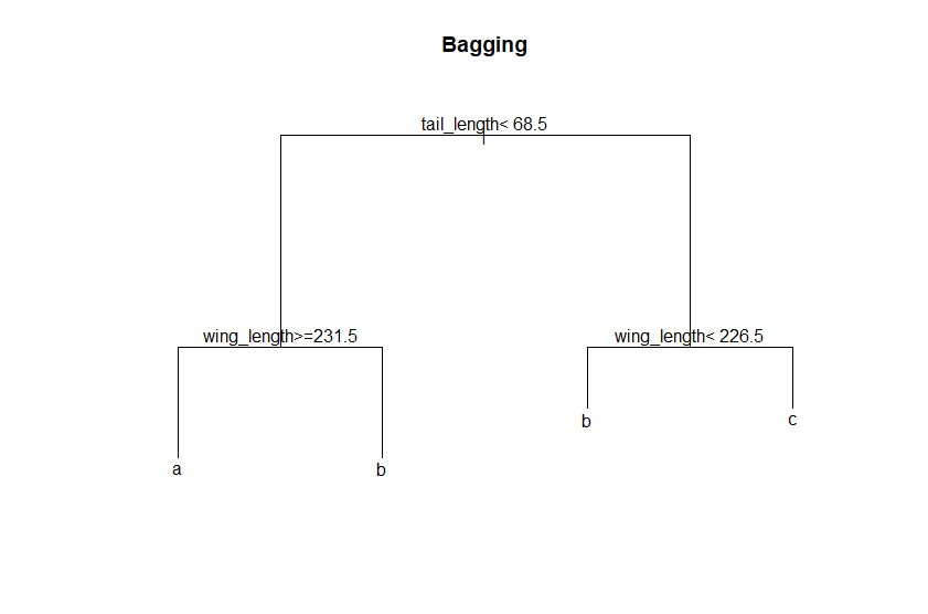
> c_bag <- bagging(breeds ~., data = c_train, type = "class")
>
> names(c_bag) # 모델 객체 확인
[1] "formula" "trees" "votes" "prob" "class" "samples" "importance" "terms" "call"
> c_bag$importance # 모델 객체 중 importance 확인
comb_height tail_length wing_length
7.303416 49.583232 43.113351
>
> # c_bag 모델의 trees 객체의 100번째 트리 그래프로 그리고, 텍스트 추가하기
> # margin의 경우 그래프에서 텍스트가 잘리는 문제가 발생해 부여함
> plot(c_bag$trees[[100]], main = "Bagging", margin=0.1)
> text(c_bag$trees[[100]])
>
> # 배깅 모델에 테스트용 데이터 셋을 이용해 품종 분류 실시
> pred <- predict(c_bag, newdata = c_test, type = "class")
> str(pred) # 예측값(class) 외에도 다양한 결과가 입력된 리스트 형태임
List of 6
$ formula :Class 'formula' language breeds ~ .
.. ..- attr(*, ".Environment")=<environment: R_GlobalEnv>
$ votes : num [1:60, 1:3] 100 100 100 100 100 25 100 100 100 100 ...
$ prob : num [1:60, 1:3] 1 1 1 1 1 0.25 1 1 1 1 ...
$ class : chr [1:60] "a" "a" "a" "a" ...
$ confusion: 'table' int [1:3, 1:3] 19 1 0 2 16 2 0 2 18
..- attr(*, "dimnames")=List of 2
.. ..$ Predicted Class: chr [1:3] "a" "b" "c"
.. ..$ Observed Class : chr [1:3] "a" "b" "c"
$ error : num 0.117
>
> # 모델의 예측값(class)만 c_test에 pred열을 만들어 입력(단, 형태는 factor로 변경)
> c_test$pred <- as.factor(pred$class)
> confusionMatrix(c_test$pred, c_test$breeds)
Confusion Matrix and Statistics
Reference
Prediction a b c
a 19 2 0
b 1 16 2
c 0 2 18
Overall Statistics
Accuracy : 0.8833
95% CI : (0.7743, 0.9518)
No Information Rate : 0.3333
P-Value [Acc > NIR] : < 2.2e-16
Kappa : 0.825
Mcnemar's Test P-Value : NA
Statistics by Class:
Class: a Class: b Class: c
Sensitivity 0.9500 0.8000 0.9000
Specificity 0.9500 0.9250 0.9500
Pos Pred Value 0.9048 0.8421 0.9000
Neg Pred Value 0.9744 0.9024 0.9500
Prevalence 0.3333 0.3333 0.3333
Detection Rate 0.3167 0.2667 0.3000
Detection Prevalence 0.3500 0.3167 0.3333
Balanced Accuracy 0.9500 0.8625 0.9250
>
>
> # (Ada)Boosting
>
> c_train <- read.csv("ch6-2_train.csv", header = TRUE)
> c_test <- read.csv("ch6-2_test.csv", header = TRUE)
> c_train$breeds <- as.factor(c_train$breeds)
> c_test$breeds <- as.factor(c_test$breeds)
>
> c_boost <- boosting(breeds ~., data = c_train, type = "class")
> c_boost$importance
comb_height tail_length wing_length
20.98737 42.70707 36.30556
>
> # 그래프 글자 잘림 방지를 위해 margin 지정
> plot(c_boost$trees[[100]], main = "Boosting-Adaboost", margin = 0.1)
> text(c_boost$trees[[100]])

>
> pred <- predict(c_boost, newdata = c_test, type = "class")
> c_test$pred <- as.factor(pred$class)
> confusionMatrix(c_test$pred, c_test$breeds)
Confusion Matrix and Statistics
Reference
Prediction a b c
a 20 1 0
b 0 18 1
c 0 1 19
Overall Statistics
Accuracy : 0.95
95% CI : (0.8608, 0.9896)
No Information Rate : 0.3333
P-Value [Acc > NIR] : < 2.2e-16
Kappa : 0.925
Mcnemar's Test P-Value : NA
Statistics by Class:
Class: a Class: b Class: c
Sensitivity 1.0000 0.9000 0.9500
Specificity 0.9750 0.9750 0.9750
Pos Pred Value 0.9524 0.9474 0.9500
Neg Pred Value 1.0000 0.9512 0.9750
Prevalence 0.3333 0.3333 0.3333
Detection Rate 0.3333 0.3000 0.3167
Detection Prevalence 0.3500 0.3167 0.3333
Balanced Accuracy 0.9875 0.9375 0.9625
>
>
> # Random Forest
>
> library(randomForest)
>
> c_train <- read.csv("ch6-2_train.csv", header = TRUE)
> c_test <- read.csv("ch6-2_test.csv", header = TRUE)
> c_train$breeds <- as.factor(c_train$breeds)
> c_test$breeds <- as.factor(c_test$breeds)
>
> c_rf <- randomForest(breeds ~., data = c_train, type = "class")
> names(c_rf)
[1] "call" "type" "predicted" "err.rate" "confusion" "votes"
[7] "oob.times" "classes" "importance" "importanceSD" "localImportance" "proximity"
[13] "ntree" "mtry" "forest" "y" "test" "inbag"
[19] "terms"
> c_rf$importance # 모델 객체 중 importance 확인
MeanDecreaseGini
wing_length 50.49929
tail_length 70.36963
comb_height 30.17979
> varImpPlot(c_rf)

>
> c_test$pred <- predict(c_rf, newdata = c_test, type = "class")
> confusionMatrix(c_test$pred, c_test$breeds)
Confusion Matrix and Statistics
Reference
Prediction a b c
a 20 1 0
b 0 18 1
c 0 1 19
Overall Statistics
Accuracy : 0.95
95% CI : (0.8608, 0.9896)
No Information Rate : 0.3333
P-Value [Acc > NIR] : < 2.2e-16
Kappa : 0.925
Mcnemar's Test P-Value : NA
Statistics by Class:
Class: a Class: b Class: c
Sensitivity 1.0000 0.9000 0.9500
Specificity 0.9750 0.9750 0.9750
Pos Pred Value 0.9524 0.9474 0.9500
Neg Pred Value 1.0000 0.9512 0.9750
Prevalence 0.3333 0.3333 0.3333
Detection Rate 0.3333 0.3000 0.3167
Detection Prevalence 0.3500 0.3167 0.3333
Balanced Accuracy 0.9875 0.9375 0.9625
>
>
> # SVM
>
> c_train <- read.csv("ch6-2_train.csv", header = TRUE) # 훈련용 데이터셋 불러오기
> c_test <- read.csv("ch6-2_test.csv", header = TRUE) # 테스트용 데이터셋 불러오기
> c_train$breeds <- as.factor(c_train$breeds)
> c_test$breeds <- as.factor(c_test$breeds)
>
> # 병아리 품종을 종속변수로 나머지 변수를 독립변수로한 학습 실시
> c_svm <- svm(breeds ~., data = c_train)
>
> plot(c_svm, c_train, wing_length ~ tail_length,
+ slice = list(comb_height = 34))

>
> c_test$pred <- predict(c_svm, newdata = c_test, type = "class")
> confusionMatrix(c_test$pred, c_test$breeds)
Confusion Matrix and Statistics
Reference
Prediction a b c
a 20 1 0
b 0 17 1
c 0 2 19
Overall Statistics
Accuracy : 0.9333
95% CI : (0.838, 0.9815)
No Information Rate : 0.3333
P-Value [Acc > NIR] : < 2.2e-16
Kappa : 0.9
Mcnemar's Test P-Value : NA
Statistics by Class:
Class: a Class: b Class: c
Sensitivity 1.0000 0.8500 0.9500
Specificity 0.9750 0.9750 0.9500
Pos Pred Value 0.9524 0.9444 0.9048
Neg Pred Value 1.0000 0.9286 0.9744
Prevalence 0.3333 0.3333 0.3333
Detection Rate 0.3333 0.2833 0.3167
Detection Prevalence 0.3500 0.3000 0.3500
Balanced Accuracy 0.9875 0.9125 0.9500
>
>
> # XGBoost, 데이터 타입을 바꿔야하고 학습이 있어야함
>
> library(xgboost)
>
> c_train <- read.csv("ch6-2_train.csv", header = TRUE)
> c_test <- read.csv("ch6-2_test.csv", header = TRUE)
> c_train$breeds <- as.factor(c_train$breeds)
> c_test$breeds <- as.factor(c_test$breeds)
>
> c_x_train <- data.matrix(c_train[,1:3]) # 훈련용 데이터 셋 matrix 타입으로 만들기
> c_y_train <- c_train[,4] # 훈련용 라벨 만들기, vector 타입
> c_x_test <- data.matrix(c_test[,1:3]) # 테스트용 데이터 셋 matrix 타입으로 만들기
> c_y_test <- c_test[,4] # 테스트용 라벨 만들기, vector 타입
> # xgboost() 함수의 경우 독립변수 데이터와 라벨(종속변수)이 분리되어야 적용이 가능
> # 특히 독립변수 데이터의 경우 matrix 타입이어야 학습이 가능
>
> # xgboost() 함수의 경우 label을 인식할 때 1부터가 아닌 0부터 인식해서 -1을 해줘야 한다.
> c_xgb <- xgboost(data = c_x_train, label = as.numeric(c_y_train)-1,
+ num_class = 3, nrounds = 20, eta = 0.1,
+ objective = "multi:softprob")
[17:21:02] WARNING: amalgamation/../src/learner.cc:1115: Starting in XGBoost 1.3.0, the default evaluation metric used with the objective 'multi:softprob' was changed from 'merror' to 'mlogloss'. Explicitly set eval_metric if you'd like to restore the old behavior.
[1] train-mlogloss:0.971105
[2] train-mlogloss:0.865701
[3] train-mlogloss:0.775503
[4] train-mlogloss:0.697766
[5] train-mlogloss:0.630219
[6] train-mlogloss:0.570131
[7] train-mlogloss:0.517825
[8] train-mlogloss:0.471655
[9] train-mlogloss:0.430063
[10] train-mlogloss:0.393037
[11] train-mlogloss:0.360194
[12] train-mlogloss:0.330842
[13] train-mlogloss:0.304554
[14] train-mlogloss:0.280966
[15] train-mlogloss:0.259756
[16] train-mlogloss:0.240658
[17] train-mlogloss:0.223431
[18] train-mlogloss:0.208234
[19] train-mlogloss:0.194523
[20] train-mlogloss:0.181680
>
> # 모델에 테스트용 데이터 셋을 넣어 예측한 후 예측값(확률)을 matrix 타입으로 변환
> c_y_test_pred <- predict(c_xgb, c_x_test, reshape = TRUE)
>
> # 모델의 예측값(확률) 중 가장 큰 값에 대응되는 라벨로 매핑
> c_y_test_pred_label <- levels(c_y_test)[max.col(c_y_test_pred)]
> class(c_y_test_pred_label)
[1] "character"
>
> # character 속성인 예측결과 라벨을 factor 속성으로 변환(factor의 경우 level이 존재)
> c_y_test_pred_label <- as.factor(c_y_test_pred_label)
>
> confusionMatrix(c_y_test_pred_label, c_y_test)
Confusion Matrix and Statistics
Reference
Prediction a b c
a 20 1 0
b 0 17 2
c 0 2 18
Overall Statistics
Accuracy : 0.9167
95% CI : (0.8161, 0.9724)
No Information Rate : 0.3333
P-Value [Acc > NIR] : < 2.2e-16
Kappa : 0.875
Mcnemar's Test P-Value : NA
Statistics by Class:
Class: a Class: b Class: c
Sensitivity 1.0000 0.8500 0.9000
Specificity 0.9750 0.9500 0.9500
Pos Pred Value 0.9524 0.8947 0.9000
Neg Pred Value 1.0000 0.9268 0.9500
Prevalence 0.3333 0.3333 0.3333
Detection Rate 0.3333 0.2833 0.3000
Detection Prevalence 0.3500 0.3167 0.3333
Balanced Accuracy 0.9875 0.9000 0.9250
>
> # nrounds 20 -> 50 조정
> c_xgb2 <- xgboost(data = c_x_train, label = as.numeric(c_y_train)-1,
+ num_class = 3, nrounds = 50, eta = 0.1,
+ objective = "multi:softprob")
[17:27:49] WARNING: amalgamation/../src/learner.cc:1115: Starting in XGBoost 1.3.0, the default evaluation metric used with the objective 'multi:softprob' was changed from 'merror' to 'mlogloss'. Explicitly set eval_metric if you'd like to restore the old behavior.
[1] train-mlogloss:0.971106
[2] train-mlogloss:0.865701
[3] train-mlogloss:0.775503
[4] train-mlogloss:0.697766
[5] train-mlogloss:0.630219
[6] train-mlogloss:0.570131
[7] train-mlogloss:0.517825
[8] train-mlogloss:0.471655
[9] train-mlogloss:0.430063
[10] train-mlogloss:0.393037
[11] train-mlogloss:0.360194
[12] train-mlogloss:0.330842
[13] train-mlogloss:0.304554
[14] train-mlogloss:0.280966
[15] train-mlogloss:0.259756
[16] train-mlogloss:0.240658
[17] train-mlogloss:0.223431
[18] train-mlogloss:0.208234
[19] train-mlogloss:0.194523
[20] train-mlogloss:0.181680
[21] train-mlogloss:0.169962
[22] train-mlogloss:0.159345
[23] train-mlogloss:0.149811
[24] train-mlogloss:0.141196
[25] train-mlogloss:0.133361
[26] train-mlogloss:0.126199
[27] train-mlogloss:0.119659
[28] train-mlogloss:0.113637
[29] train-mlogloss:0.108158
[30] train-mlogloss:0.102891
[31] train-mlogloss:0.098194
[32] train-mlogloss:0.093550
[33] train-mlogloss:0.089555
[34] train-mlogloss:0.085887
[35] train-mlogloss:0.082514
[36] train-mlogloss:0.079247
[37] train-mlogloss:0.076433
[38] train-mlogloss:0.073629
[39] train-mlogloss:0.071167
[40] train-mlogloss:0.068891
[41] train-mlogloss:0.066424
[42] train-mlogloss:0.064144
[43] train-mlogloss:0.062021
[44] train-mlogloss:0.060047
[45] train-mlogloss:0.058196
[46] train-mlogloss:0.056623
[47] train-mlogloss:0.055080
[48] train-mlogloss:0.053533
[49] train-mlogloss:0.052246
[50] train-mlogloss:0.051148
>
> # 모델에 테스트용 데이터 셋을 넣어 예측한 후 예측값(확률)을 matrix 타입으로 변환
> c_y_test_pred2 <- predict(c_xgb2, c_x_test, reshape = TRUE)
>
> # 모델의 예측값(확률) 중 가장 큰 값에 대응되는 라벨로 매핑
> c_y_test_pred_label2 <- levels(c_y_test)[max.col(c_y_test_pred2)]
>
> # character 속성인 예측결과 라벨을 factor 속성으로 변환
> c_y_test_pred_label2 <- as.factor(c_y_test_pred_label2)
>
> confusionMatrix(c_y_test_pred_label2, c_y_test)
Confusion Matrix and Statistics
Reference
Prediction a b c
a 20 1 0
b 0 18 2
c 0 1 18
Overall Statistics
Accuracy : 0.9333
95% CI : (0.838, 0.9815)
No Information Rate : 0.3333
P-Value [Acc > NIR] : < 2.2e-16
Kappa : 0.9
Mcnemar's Test P-Value : NA
Statistics by Class:
Class: a Class: b Class: c
Sensitivity 1.0000 0.9000 0.9000
Specificity 0.9750 0.9500 0.9750
Pos Pred Value 0.9524 0.9000 0.9474
Neg Pred Value 1.0000 0.9500 0.9512
Prevalence 0.3333 0.3333 0.3333
Detection Rate 0.3333 0.3000 0.3000
Detection Prevalence 0.3500 0.3333 0.3167
Balanced Accuracy 0.9875 0.9250 0.9375
>
> # eta 0.1 -> 0.3 조정
> c_xgb3 <- xgboost(data = c_x_train, label = as.numeric(c_y_train)-1,
+ num_class = 3, nrounds = 50, eta = 0.3,
+ objective = "multi:softprob")
[17:30:41] WARNING: amalgamation/../src/learner.cc:1115: Starting in XGBoost 1.3.0, the default evaluation metric used with the objective 'multi:softprob' was changed from 'merror' to 'mlogloss'. Explicitly set eval_metric if you'd like to restore the old behavior.
[1] train-mlogloss:0.745592
[2] train-mlogloss:0.540153
[3] train-mlogloss:0.403320
[4] train-mlogloss:0.308994
[5] train-mlogloss:0.242033
[6] train-mlogloss:0.193549
[7] train-mlogloss:0.158481
[8] train-mlogloss:0.131042
[9] train-mlogloss:0.110702
[10] train-mlogloss:0.095217
[11] train-mlogloss:0.083322
[12] train-mlogloss:0.074003
[13] train-mlogloss:0.066380
[14] train-mlogloss:0.059571
[15] train-mlogloss:0.054102
[16] train-mlogloss:0.049925
[17] train-mlogloss:0.046737
[18] train-mlogloss:0.044114
[19] train-mlogloss:0.041775
[20] train-mlogloss:0.039940
[21] train-mlogloss:0.038209
[22] train-mlogloss:0.036996
[23] train-mlogloss:0.035606
[24] train-mlogloss:0.034645
[25] train-mlogloss:0.033884
[26] train-mlogloss:0.032949
[27] train-mlogloss:0.032197
[28] train-mlogloss:0.031416
[29] train-mlogloss:0.030825
[30] train-mlogloss:0.030327
[31] train-mlogloss:0.029836
[32] train-mlogloss:0.029306
[33] train-mlogloss:0.028917
[34] train-mlogloss:0.028513
[35] train-mlogloss:0.028058
[36] train-mlogloss:0.027746
[37] train-mlogloss:0.027422
[38] train-mlogloss:0.027098
[39] train-mlogloss:0.026807
[40] train-mlogloss:0.026567
[41] train-mlogloss:0.026329
[42] train-mlogloss:0.026147
[43] train-mlogloss:0.025950
[44] train-mlogloss:0.025736
[45] train-mlogloss:0.025527
[46] train-mlogloss:0.025376
[47] train-mlogloss:0.025190
[48] train-mlogloss:0.025083
[49] train-mlogloss:0.024941
[50] train-mlogloss:0.024705
>
> # 모델에 테스트용 데이터 셋을 넣어 예측한 후 예측값(확률)을 matrix 타입으로 변환
> c_y_test_pred3 <- predict(c_xgb3, c_x_test, reshape = TRUE)
>
> # 모델의 예측값(확률) 중 가장 큰 값에 대응되는 라벨로 매핑
> c_y_test_pred_label3 <- levels(c_y_test)[max.col(c_y_test_pred3)]
>
> # character 속성인 예측결과 라벨을 factor 속성으로 변환
> c_y_test_pred_label3 <- as.factor(c_y_test_pred_label3)
>
> confusionMatrix(c_y_test_pred_label3, c_y_test)
Confusion Matrix and Statistics
Reference
Prediction a b c
a 20 1 0
b 0 18 1
c 0 1 19
Overall Statistics
Accuracy : 0.95
95% CI : (0.8608, 0.9896)
No Information Rate : 0.3333
P-Value [Acc > NIR] : < 2.2e-16
Kappa : 0.925
Mcnemar's Test P-Value : NA
Statistics by Class:
Class: a Class: b Class: c
Sensitivity 1.0000 0.9000 0.9500
Specificity 0.9750 0.9750 0.9750
Pos Pred Value 0.9524 0.9474 0.9500
Neg Pred Value 1.0000 0.9512 0.9750
Prevalence 0.3333 0.3333 0.3333
Detection Rate 0.3333 0.3000 0.3167
Detection Prevalence 0.3500 0.3167 0.3333
Balanced Accuracy 0.9875 0.9375 0.9625
출처 : 현장에서 바로 써먹는 데이터 분석 with R
'데이터분석 > R' 카테고리의 다른 글
| [현장에서 바로 써먹는...] 인공신경망과 딥러닝 - 회귀 (0) | 2022.04.13 |
|---|---|
| [현장에서 바로 써먹는...] 군집분석 (0) | 2022.04.09 |
| [현장에서 바로 써먹는...] 로지스틱 회귀 (0) | 2022.04.09 |
| [현장에서 바로 써먹는...] 회귀분석 (0) | 2022.04.07 |
| [현장에서 바로 써먹는...] 상관분석 (0) | 2022.04.05 |


