> ## Chapter 7-2. 딥 러닝을 이용해 병아리 품종을 다시 구분 해보자 (분류)
>
> # Keras 활용 딥러닝
>
> install.packages("keras") # keras 패키지 설치
> install.packages("tensorflow") # tensorflow 패키지 설치
> library(keras) # keras 라이브러리 불러오기
> install_keras() # keras 설치
> library(tensorflow) # tensorflow 라이브러리 불러오기
> install_tensorflow() # tensorlfow 설치
>
> # 데이터 불러오기
> c_train <- read.csv("ch6-2_train.csv", header = TRUE)
> c_test <- read.csv("ch6-2_test.csv", header = TRUE)
>
> c_x_train <- c_train[,1:3] # 훈련용 데이터 셋 만들기
> c_y_train <- c_train[,4] # 훈련용 라벨 만들기, vector 타입
> c_x_test <- c_test[,1:3] # 테스트용 데이터 셋 만들기
> c_y_test <- c_test[,4] # 테스트용 라벨 만들기, vector 타입
>
> str(c_x_train)
'data.frame': 240 obs. of 3 variables:
$ wing_length: int 238 236 256 240 246 233 235 241 232 234 ...
$ tail_length: int 63 67 65 63 65 65 66 66 64 64 ...
$ comb_height: int 34 30 34 35 30 30 30 35 31 30 ...
>
> # caret 패키지에서 preProcess() 함수로 스케일링을 제공하기 때문에 불러옴
> library(caret)
>
> # preProcess() 함수에서 method를 range로 지정하면 Normalization 가능
> nor <- preProcess(c_x_train[,1:3], method="range")
>
> # predict() 함수를 이용해 c_x_train 데이터를 Normalization 실시
> n_c_x_train <- predict(nor, c_x_train)
> summary(n_c_x_train) # Normalization 결과 확인
wing_length tail_length comb_height
Min. :0.0000 Min. :0.0000 Min. :0.0000
1st Qu.:0.3469 1st Qu.:0.3333 1st Qu.:0.3750
Median :0.5102 Median :0.5000 Median :0.5000
Mean :0.5124 Mean :0.5069 Mean :0.5089
3rd Qu.:0.7194 3rd Qu.:0.7500 3rd Qu.:0.7500
Max. :1.0000 Max. :1.0000 Max. :1.0000
>
> # predict() 함수를 이용해 c_x_test 데이터를 Normalization 실시
> n_c_x_test <- predict(nor, c_x_test)
> summary(n_c_x_test) # Normalization 결과 확인
wing_length tail_length comb_height
Min. :0.0000 Min. :0.0000 Min. :0.0000
1st Qu.:0.3622 1st Qu.:0.3125 1st Qu.:0.3750
Median :0.5612 Median :0.5417 Median :0.5000
Mean :0.5507 Mean :0.5319 Mean :0.5083
3rd Qu.:0.7959 3rd Qu.:0.7500 3rd Qu.:0.6250
Max. :1.0000 Max. :1.0000 Max. :1.0000
>
> # Matrix 형태로 변환
> n_c_x_train <- as.matrix(n_c_x_train)
> n_c_x_test <- as.matrix(n_c_x_test)
>
> c_y_train <- as.factor(c_y_train)
> c_y_test <- as.factor(c_y_test)
>
> # 종속변수 a, b, c를 각각 0, 1, 2 숫자로 변환
> nu_c_y_train <- as.numeric(c_y_train) -1
> nu_c_y_test <- as.numeric(c_y_test) -1
>
> class(n_c_x_train) # 데이터 형태 확인
[1] "matrix" "array"
> class(nu_c_y_train) # 데이터 형태 확인
[1] "numeric"
> head(nu_c_y_train) # 문자가 숫자로 잘 변환되었는지 확인
[1] 0 0 0 0 0 0
> str(nu_c_y_train)
num [1:240] 0 0 0 0 0 0 0 0 0 0 ...
>
> # One-hot encoding 위해 필요
> # (keras라이브러리) 라벨 One-hot encoding
> o_c_y_train <- to_categorical(nu_c_y_train)
> o_c_y_test <- to_categorical(nu_c_y_test)
>
> head(o_c_y_train)
[,1] [,2] [,3]
[1,] 1 0 0
[2,] 1 0 0
[3,] 1 0 0
[4,] 1 0 0
[5,] 1 0 0
[6,] 1 0 0
> tail(o_c_y_train)
[,1] [,2] [,3]
[235,] 0 0 1
[236,] 0 0 1
[237,] 0 0 1
[238,] 0 0 1
[239,] 0 0 1
[240,] 0 0 1
>
> # 모델(model) 생성
> model <- keras_model_sequential()
>
> #모델에 계층 추가
> model %>%
+ layer_dense(units = 16, activation = 'relu', input_shape = 3) %>%
+ layer_dense(units = 16, activation = 'relu') %>%
+ layer_dense(units = 3, activation = 'softmax')
> # input_shape : 입력층의 크기로 n_c_x_train 데이터 셋의 독립변수가 3개이므로 3 입력
> # units : 층의 노드 갯수로 일반적으로 은닉층의 경우 4의 배수를 주로 사용하고 출력층의 경우 분류 문제에서는 최종 분류 결과의 갯수만큼 설정하고, 회귀 문제에서는 1로 설정
> # activation : 활성화 함수로 은닉층의 경우 주로 relu, tanh를 사용하고 출력층의 경우 이진 분류에서는 sigmoid, 다중 분류에서는 softmax, 회귀에서는 linear 또는 생략
>
> # 모델 살펴보기
> summary(model)
Model: "sequential"
____________________________________________________________________________________________________________________________
Layer (type) Output Shape Param #
============================================================================================================================
dense_2 (Dense) (None, 16) 64
____________________________________________________________________________________________________________________________
dense_1 (Dense) (None, 16) 272
____________________________________________________________________________________________________________________________
dense (Dense) (None, 3) 51
============================================================================================================================
Total params: 387
Trainable params: 387
Non-trainable params: 0
____________________________________________________________________________________________________________________________
> # 첫번째 은닉층인 dense_2의 경우는 3개의 입력값과 16개 노드의 모든 조합으로 가능한 가중치(weight) 48(3*16)개와 절편(bias) 16개가 합쳐져 총 64개의 파라미터가 존재한다.
> # 두번째 은닉층인 dense_1의 경우는 첫번째 은닉층의 결과 16개와 16개 노드의 모든 조합으로 가능한 가중치 256개와 절편 16개가 합쳐져 총 272개의 파라미터가 존재한다.
>
>
> # 모델 학습설정(compile)
> model %>% compile(
+ loss = 'categorical_crossentropy',
+ optimizer = 'adam',
+ metrics = 'accuracy'
+ )
> # loss : 손실 함수로 신경망의 성능을 나타내는 지표인데 낮을수록 좋으며 이진 분류일 경우 binary_crossentropy, 다중 분류일 경우 catogorical_crossentropy, 회귀일 경우 mse, mae를 주로 사용
> # optimizer : 최적화기로 손실 함수의 값을 최소로 하는 가중치(weight) 최적값을 찾아가는 도구인데 Keras에서는 SGD, RMSprop, Adagrad, Adadelta, Adamax, Nadam, Adam을 사용할 수 있으며 일반적으로 Adam이 높은 성능을 나타내는 경우가 많음
> # metrics : 평가 지표로 학습하는 동안 모델의 성능을 평가하는 지표인데 분류 문제에서는 accuracy, 회귀 문제에서는 mse, mae, rmse 등을 주로 사용
>
> # 모델 학습 실시
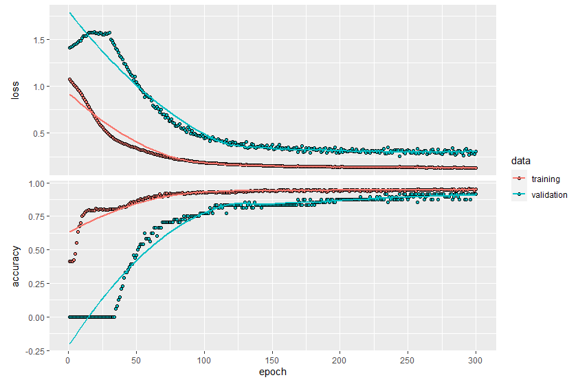
> history <- model %>% fit(
+ n_c_x_train,
+ o_c_y_train,
+ epochs = 300,
+ batch_size = 16,
+ validation_split = 0.2
+ )
2022-04-20 06:19:00.234084: I tensorflow/compiler/mlir/mlir_graph_optimization_pass.cc:185] None of the MLIR Optimization Passes are enabled (registered 2)
Epoch 1/300
12/12 [==============================] - 1s 15ms/step - loss: 1.0760 - accuracy: 0.4167 - val_loss: 1.4068 - val_accuracy: 0.0000e+00end` is slow compared to the batch time (batch time: 0.0004s vs `on_train_batch_end` time: 0.0007s). Check your callbacks.
Epoch 2/300
12/12 [==============================] - 0s 3ms/step - loss: 1.0545 - accuracy: 0.4167 - val_loss: 1.4157 - val_accuracy: 0.0000e+00
...
Epoch 299/300
12/12 [==============================] - 0s 2ms/step - loss: 0.1323 - accuracy: 0.9427 - val_loss: 0.2772 - val_accuracy: 0.9167
Epoch 300/300
12/12 [==============================] - 0s 2ms/step - loss: 0.1303 - accuracy: 0.9531 - val_loss: 0.3063 - val_accuracy: 0.9167

> # epochs : 학습 횟수로 너무 부족하면 과소적합이 될 수 있고, 너무 많이 하면 학습 시간이 오래 걸리고 과적합이 될 수 있음
> # batch_size : 배치 크기로 한번에 학습할 데이터의 크기를 말하며 240개의 학습용 데이터가 있을 때 batch_size가 16이면 15개로 분할해서 학습을 실시하며 이때 15번의 가중치 갱신이 일어남
> # validation_split : 검증(validation)에 사용할 데이터의 비율을 설정하는 것으로 240개의 학습용 데이터가 있을 때 0.2로 지정하면 48개는 검증용으로 사용하고, 나머지 192개를 학습용으로 사용
>
> # 학습과정 그래프 표시
> plot(history)
`geom_smooth()` using formula 'y ~ x'
>
> # 테스트 데이터셋을 이용한 분류성능 평가
> pred_mat <- model %>% predict(n_c_x_test)
> head(pred_mat) # 데이터 확인
[,1] [,2] [,3]
[1,] 0.9987367 3.624622e-05 1.227169e-03
[2,] 0.9999962 1.658489e-06 2.101144e-06
[3,] 0.9999980 1.725506e-06 3.469380e-07
[4,] 0.9999967 2.876311e-06 4.261259e-07
[5,] 0.9999995 5.206480e-07 4.450780e-08
[6,] 0.9838695 1.610988e-02 2.062355e-05
>
> # 확률값에 따라 a, b, c로 결과 매핑
> pred_mat_label <- levels(c_y_test)[max.col(pred_mat)]
> head(pred_mat_label) # 데이터 확인
[1] "a" "a" "a" "a" "a" "a"
>
> pred <- as.factor(pred_mat_label) # 예측값 factor로 타입 변경
> act <- as.factor(c_y_test) # 실제값 factor로 타입 변경
>
> # 정오분류표(Confusion Matrix) 생성
> confusionMatrix(pred, act)
Confusion Matrix and Statistics
Reference
Prediction a b c
a 20 1 0
b 0 17 1
c 0 2 19
Overall Statistics
Accuracy : 0.9333
95% CI : (0.838, 0.9815)
No Information Rate : 0.3333
P-Value [Acc > NIR] : < 2.2e-16
Kappa : 0.9
Mcnemar's Test P-Value : NA
Statistics by Class:
Class: a Class: b Class: c
Sensitivity 1.0000 0.8500 0.9500
Specificity 0.9750 0.9750 0.9500
Pos Pred Value 0.9524 0.9444 0.9048
Neg Pred Value 1.0000 0.9286 0.9744
Prevalence 0.3333 0.3333 0.3333
Detection Rate 0.3333 0.2833 0.3167
Detection Prevalence 0.3500 0.3000 0.3500
Balanced Accuracy 0.9875 0.9125 0.9500
>
>
> # (참고)Dropout용 모델(model) 생성
> model_d <- keras_model_sequential()
>
> # 모델에 계층 추가(Dropout 40% 적용)
> model_d %>%
+ layer_dense(units = 16, activation = 'relu', input_shape = 3) %>%
+ layer_dropout(rate = 0.4) %>%
+ layer_dense(units = 16, activation = 'relu') %>%
+ layer_dropout(rate = 0.4) %>%
+ layer_dense(units = 3, activation = 'softmax')
>
> # 모델 살펴보기
> summary(model_d)
Model: "sequential_1"
____________________________________________________________________________________________________________________________
Layer (type) Output Shape Param #
============================================================================================================================
dense_5 (Dense) (None, 16) 64
____________________________________________________________________________________________________________________________
dropout_1 (Dropout) (None, 16) 0
____________________________________________________________________________________________________________________________
dense_4 (Dense) (None, 16) 272
____________________________________________________________________________________________________________________________
dropout (Dropout) (None, 16) 0
____________________________________________________________________________________________________________________________
dense_3 (Dense) (None, 3) 51
============================================================================================================================
Total params: 387
Trainable params: 387
Non-trainable params: 0
____________________________________________________________________________________________________________________________
출처 : 현장에서 바로 써먹는 데이터 분석 with R
'데이터분석 > R' 카테고리의 다른 글
| [현장에서 바로 써먹는...] 텍스트마이닝 - 워드클라우드 (0) | 2022.05.02 |
|---|---|
| 타이타닉 데이터 분류 예측 (0) | 2022.04.25 |
| [현장에서 바로 써먹는...] 인공신경망과 딥러닝 - 회귀 (0) | 2022.04.13 |
| [현장에서 바로 써먹는...] 군집분석 (0) | 2022.04.09 |
| [현장에서 바로 써먹는...] 분류분석 (0) | 2022.04.09 |


